High frequency transmission lines

Introduction

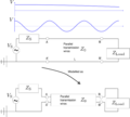
Antenna system.

Lähetin, johto, antenni, jne. https://www.antenna-theory.com/tutorial/txline/transmissionline.php

https://www.worldradiohistory.com/BOOKSHELF-ARH/Technology/Rider-Books/R-F%20Transmission%20Lines%20-%20Alexander%20Schure.pdf

Transmission line, general case

• 

  The (long) transmission line is modeled as Z₀. If the frequency (wavelength) of the source is too large (small) compared to dimensions of the system, it need to be considered in more detailed. See also the svg file.

• 

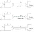
  The physical realizations of the transmission lines are usually coaxial cables, twisted cables or twin lead cables.

• 

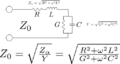
  The system is analyzed as being differential short pieces. The conductance $G$ is the conductance between the two wires, which exists because of the high frequency.

General case

If a transmission line has a length greater than about 10% of a wavelength, then the line length will noticeably affect the circuit's impedance. The equation in the above image can be written as

${\begin{aligned}{\frac {\partial v}{dx}}&=-L{\frac {\partial i}{\partial t}}-Ri\\{\frac {\partial i}{dx}}&=-C{\frac {\partial v}{\partial t}}-Gv\end{aligned}}$

and these two is easy to combine, and it gives the second degree dy

${\frac {\partial ^{2}v}{dx^{2}}}-LC{\frac {\partial ^{2}v}{\partial t^{2}}}=(RC+GL){\frac {\partial v}{\partial t}}+GRv$

and similar equation to i. Those are damped, dispersive hyperbolic partial differential equations each involving only one unknown. Lets solve those. (Telegrapher's equations)

Lossless transmission

If wire resistance and insulation conductance can be neglected (R=G=0), the model depends only on L and C elements. Thus, we have two similar wave equations for v and i (only for v is shown)

${\frac {\partial ^{2}v}{\partial ^{2}t^{2}}}-{\hat {v}}^{2}{\frac {\partial v}{\partial x^{2}}}=0$

where ${\hat {v}}=(LC)^{-1/2}$. These reduce to one-dimensional Helmholtz equations, or eigenmodes, and the result if an eigenmode is

${\begin{aligned}v_{\omega }(x)&=v^{+}e^{-\imath (kx+\omega t)}+v^{-}e^{+\imath (kx-\omega t)}\\i_{\omega }(x)&={\frac {v^{+}}{Z_{0}}}e^{-\imath (kx+\omega t)}+{\frac {v^{-}}{Z_{0}}}e^{+\imath (kx-\omega t)}\end{aligned}}$

where k is the wave number $k=\omega {\sqrt {LC}}$ and $Z_{0}$ is the characteristic impedance, which for the lossles transmission line is

$Z_{0}={\sqrt {\frac {L}{Z}}}$

The full solution can be decomposed into an eigenmode expansion $u(x,t)=\int _{-\infty }^{\infty }s(\omega )v_{\omega }(x,t)d\omega$

Frequency Domain

${\begin{aligned}{\frac {dv_{\omega }}{dx}}&=-(\imath \omega L_{\omega }+R_{\omega })i_{\omega }(x)\\\%{\frac {di_{\omega }}{dx}}&=-(\imath \omega C_{\omega }+G_{\omega })v_{\omega }(x)\\\end{aligned}}$

and by combining these we get

${\frac {d^{2}v_{\omega }}{dx^{2}}}=\gamma ^{2}v_{\omega }$

and similar for $i$, with $\gamma =\alpha +\imath b={\sqrt {(R_{\omega }+\imath \omega L_{\omega })(G_{\omega }+\imath \omega C_{\omega })}}$

S

The solutions to the above equations is the sum of forward and backward traveling (reflected) waves: $v(z,t)=v^{+}e^{-\alpha z}e^{\imath (\omega t-\gamma z)}+v^{-}e^{\alpha z}e^{\imath (\omega t+\gamma z)}$ and if we assume that $\alpha =0$ we have the telegraphers equations https://en.wikipedia.org/wiki/Telegrapher's_equations

$v(z,t)=v^{+}e^{\imath (\omega t-\gamma z)}+v^{-}e^{\imath (\omega t+\gamma z)}$ and a similar for $i=i(z,t)$. If we replace $i$ by Ohm law, we get

$i(z,t)={\frac {v^{+}}{Z_{0}}}e^{\imath (\omega t-\gamma z)}+{\frac {v^{-}}{Z_{0}}}e^{\imath (\omega t+\gamma z)}={\frac {v^{+}}{Z_{0}}}e^{\imath (\omega t-\gamma z)}\left(1-{\frac {v^{-}}{v^{+}}}e^{\imath (2\gamma z)}\right)$

The fraction ${\frac {v^{-}}{v^{+}}}$ is called reflection coefficient $\Gamma$

${\frac {v^{-}}{v^{+}}}=\Gamma e^{\imath \phi _{z}}={\frac {Z_{L}-Z_{0}}{Z_{L}+Z_{0}}}$

which gives

$i(z,t)=={\frac {v^{+}}{Z_{0}}}e^{\imath (\omega t-\gamma z)}\left(1-\Gamma e^{\imath (\phi _{z}+2\gamma z)}\right)$

The characteristic impedance is

Thus we have ${\frac {d^{2}v}{dL^{2}}}=\gamma ^{2}v$ and similar for the current. The constant $\gamma ^{2}=(R+\imath \omega L)(G+\imath \omega C)$.

$Z_{0}={\frac {v^{+}}{i^{+}}}=-{\frac {v^{-}}{i^{-}}}={\sqrt {\frac {R'+\imath \omega L'}{G'+\imath \omega C'}}}$

For lossless line $R'=G'=0$ and for distortionless line $R'/L'=G'/C'$. The voltage reflection coefficient $\Gamma$

$\Gamma ={\frac {v^{-}}{v^{+}}}=-{\frac {i^{-}}{i^{+}}}={\frac {Z_{L}-Z_{0}}{Z_{L}+Z_{0}}}$ where $Z_{0}$ is the characteristic impedance of transient line, and $Z_{L}$ is the impedance of load (antenna). If $Z_{L}=Z_{0}$, then the line is perfectly matched, and there is no mismatch loss and all power is transferred to the load (antenna).

• An open circuit: $Z_{L}=\infty$ and $\Gamma =+1$.
• A short circuit: $Z_{L}=0$ and $\Gamma =-1$, and a phase reversal of the reflected voltage wave.
• A matched load: $Z_{L}=Z_{0}$, and $\Gamma =0$ and no reflections.

The voltage standing wave ratio or VSWR

${\text{VSWR}}={\frac {|V|_{\text{max}}}{||V|_{\text{min}}|}}={\frac {1+|\Gamma |}{1-|\Gamma |}}$

Siirtolinja (transmission line). Impedanssi. Koaksaalikaapelin impedanssi muodostuu sen kapasitiivisestä rakenteesta. Ei juuri resistiivistä häviötä (impedanssia) https://electronics.stackexchange.com/questions/543100/derivation-of-resistance-of-coaxial-cable. Koaksaalikaapelin ε^r

• 76.7 Ω
• 30 Ω
• The impedance of a centre-fed dipole antenna in free space is 73 Ω, so 75 Ω coax is commonly used for connecting shortwave antennas to receivers.
• Sometimes 300 Ω folded dipole antenna => 4:1 balun transformer is used.

twin-lead transmission lines: the characteristic impedance of is roughly 300 Ω.

Feeding length.

Some transmission lines are

• Coaxial cable
• Two-wire cable
• Microstrip line
• . . .

Skin Effect

The skin effect $\delta$. The higher the frequency, the more the currents are confined to the surface.

Velocity factor

Caption text

Velocity factor	Line type
0.95	Ladder line
0.82	Twin-lead
0.79	coaxial cable (foam dielectric)
0.75	RG-6 and RG-8 coaxial (thick)
0.66	RG-58 and RG-59 coaxial (thin)