AIS visualization TASK

Introduction

• 

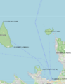
  The map and some coordinates

• 

  The map shall be transformed to photo

The position of vessels on a photo.

Data acquisition

USE RTL-AIS, ship162 (https://github.com/xoolive/ship162) project and Python, with tape measure antenna.

Or GNU AIS saves the data to local MySQL server.

Transform

Some ideas to generate the transformation. Full camera projection is not needed here.

The latitude/longitude scale is not a linear measure. Thus, to a conversion to metric scale is better. UTM projection (pyproj) or using a local tangent plane. The UTM projection works better for this 10-20 km distances.

Plan

The coordinate system of the map is WGS84 EPS:4326 to EPSG:32635.

The mapping and ideas

1. Get the mapping ship's GNSS coordinates to image coordinates
   1. Convert GNSS coordinates to UTM and then to metric points. Change the origin such that the metric numbers are reasonable.
   2. Find the corresponding pixels at the photo image.
   3. Compute homography matrix
2. For testing purposes plot the GNSS value on the map.
   1. Create other homology mapping between GNSS coordinates and the map

UTM projection

The latitude/longitude scale is not a linear measure. Thus, to a conversion to metric scale is better. UTM projection (pyproj) or using a local tangent plane. The UTM projection works better for this 10-20 km distances.

# WGS84 GPS -> UTM zone 35N
transformer = Transformer.from_crs(
    "EPSG:4326",
    "EPSG:32635",
    always_xy=True
)


gps_points = np.array([
[59.4480442,24.7727679],
[59.4720746,24.7267166],
[59.5183884,24.7962952],
[59.5226077,24.5841614],
[59.5770763,24.7294084]
])

utm_points = []
for lon, lat in gps_points:
    x, y = transformer.transform(lon, lat)
    utm_points.append([x, y])

x0, y0 = utm_points[2]
local_points = []
for x, y in utm_points:
    local_points.append([x - x0, y - y0])

print(local_points)

Homology

https://docs.opencv.org/4.x/d9/dab/tutorial_homography.html

The simplest; ${\begin{bmatrix}u\\v\\1\end{bmatrix}}{\tilde {=}}H{\begin{bmatrix}x\\y\\1\end{bmatrix}}$

Should have some 10-50 corresponding pairs to get the mapping correct. Use least squares or SVD, but OpenCV works with RANSAC.

Non rigid spatial warp

Thin plate spline, $(u,v)=f(x,y)$ where $f(x,y)=a_{1}+a_{2}x+a_{3}z+\sum _{i}w_{i}U(|p-p_{i}|)$ and $U(r)=r^{2}\log r$