Sinuosity of Kemijoki

Introduction

Use Python to estimate the sinuosity of Kemijoki.

The river was obtained from https://download.geofabrik.de/europe/finland.html but only one river (Kemijoki) with one branch is used. The extracting method is described elsewhere.

Kemijoki

• 

  Kemijoki is 550 km long according to Wikipedia. This dataset contains 500.20 km of river.

• 

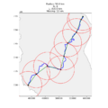
  Kemijoki measured with 50 km measure stick. The distance doesn't exactly match up, and the last 12 km is missing.

• 

  By cutting the measuring stick to half, we get one measure (25 km) more length. It still skips many of the meandering.

• 

  More distance and curves are achieved.

• 

  Missing only 1 km, but because the river curves so eccentric, it skips many kilmometers. By zooming it is easy to see that a lot of meandering is missing.

• 

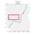
  Taking 2.5 km out of the measuring stick, we gain 30 km of river length.

• 

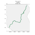
  Finally, using a 100 m strides we will arrive rather close to the GIS measure.

• 

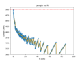
  The length vs radius. Note the sawtooth phenomena.

• 

  The fractal dimension of Kemijoki. There are different regions.

Load Data Files

import geopandas as gpd

finland = gpd.read_file("fi.shp")
finland = finland.to_crs(epsg=3067)
river = gpd.read_parquet("kemijoki_mainbranch.parquet")

Convert to points

from shapely.geometry import Point

line = river.geometry.iloc[0]
current_point = Point(line.coords[0])
points = [current_point]

Find the Intersection of the river and circle

for _ in range(50000):
     circle = current.buffer(radius)
     inter = line.intersection(circle)

     if inter.is_empty:
        break

     candidates = extract_candidate_points(inter)
     if not candidates:
        print("Error: No Candidates")
        break
     next_point = max(candidates, key=lambda p: line.project(p))

     # stop condition based on progression along line
     if line.project(next_point) <= line.project(current) + 1e-6:
        print("Error: Too close to the previous point")
        break

     current = next_point
     points.append(current)

The extract_candidates function is

Theory

Douglas-Peucker simplification at different tolerances

Fractal Dimension

The fractal dimension is defined by $L(\epsilon )=k\times \epsilon ^{1-d}$

which gives

$\log L(\epsilon )=\log k+(1-d)\log \epsilon$

The corresponding plot is called a Richardson plot.

from scipy.stats import linregress
import numpy as np

#Plot everything
plt.plot( np.log(df["R"]), np.log(df["Length (km)"])) #x, y
plt.xlabel("log (R [km])")
plt.ylabel("log(Length [km])")

#Regression
Rvalue = [2, 6, 8, 10, 13]
xmin = Rvalue[0]
for xmax in Rvalue[1:]:
    mask = (df["R"] > np.exp(xmin)) & (df["R"] < np.exp(xmax))
    x = np.log(df.loc[mask, "R"].values)             # log(epsilon)
    y = np.log(df.loc[mask, "Length (km)"].values)   # log(length)
    slope, intercept, _, _, _ = linregress(x, y)
    x_line = np.linspace(x[0], x[-1], 100)
    y_line = slope * x_line + intercept
    plt.plot(x_line, y_line, color='red', label="Fit line")
    plt.text(x[0], y[0], 'd='+ str(round(1-slope, 2)))

    print( xmin, xmax )
    xmin = xmax

plt.title("log-log Length vs R")
plt.show()

References

https://www.tud.ttu.ee/web/dmitri.kartofelev/YFX1560/Loeng_14no_vid.pdf

https://preview-www.nature.com/articles/s41598-021-85405-0.pdf