Velocity, acceleration and jerk

Introduction

The Newton $F=ma$ force rule states that force and acceleration are proportionally related. Is it possible to accelerate without noticing the jerk? The method is used in elevators, for example, and hopefully in modern (electric) cars.

We consider the acceleration the robot is subjected to while accelerating it using different acceleration functions.

Robot

Almost any robot will be ok, we use Asimov 2/ Verne.

Sensor

The Vernier acceleration sensor with the NXT Adapter is used. The sensor is attached to port number 4.

Very simple test program to see what are the measured values is shown below. The values are in arbitrary scale, and need to be normalized. We found, that the

#!/usr/bin/env python3
# https://sites.google.com/site/ev3devpython/

from ev3dev2.sensor import *
from ev3dev2.sensor import INPUT_4

import time
import os
import csv 

os.system('setfont Lat15-TerminusBold32x16')  # Try this larger font

p = Sensor( INPUT_4 )
p.mode="ANALOG-1"

def measureAcc(p):
    acc = p.value(0)
    return acc

f = open('acc.csv',"w")
writer = csv.writer(f) 
tstep = 0.001

while True:
    acc = measureAcc(p)
    print( acc )
    writer.writerow((time.time(), acc ))
    time.sleep( tstep )

The resulted file acc.csv is then manually downloaded into a computer, and plotted using Python Pandas:

import pandas as pd
import matplotlib.pyplot as plt

# Read CSV file into DataFrame df
df = pd.read_csv('acc.csv', index_col=0)

# Show thedataframe
print(df)
plt.plot(df)

Theory

The time derivative of position is velocity, then we have acceleration, and the derivative of acceleration is called jerk, $j$. ${\frac {da}{dt}}=j$ Then we have snap, crackle and pop.

See the Wikipedia page on the physiological_effects of jerk. Anyway, there might be jerky rides.

We measure the acceleration of robot, and use a numerical differential method to estimate the jerk. We use the symmetric differential;

$j(t)={\frac {da}{dt}}={\frac {f(t-h)+f(t+h)}{2h}}$ in which the first-order error cancels, and the error is $-{\frac {1}{6}}f^{(3)}(x)h^{2}$ where $t-h<x<t+h$.

We will start from zero to $t_{0}=5000$ ms where the speed should be at maximum value, $L=100$.

Standard Scheme

The ev3dev Python standard scheme is . . .

Linear acceleration

$v(t)={\begin{cases}{\frac {L}{t_{0}}}t&&{\text{if }}t<t_{0}\\L&&{\text{if }}t\geq t_{0}\end{cases}}$

because the continuity constraint $at_{0}=L$ gives that $a=L/t_{0}$.

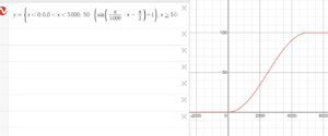
Sinusoidal acceleration

Sine acceleration

The sine curve is a harmonic motion between -1 and 1 with period $2\pi$. We use only one period, and scale that to correct acceleration function. The sine accelerates rather smoothly.

$v(t)={\begin{cases}{\frac {L}{2}}(\sin({\frac {\pi }{t_{0}}}t-{\frac {\pi }{2}})+1)&&{\text{if }}t<t_{0}\\L&&{\text{if }}t\geq t_{0}\end{cases}}$

See the interactive Desmos graph.

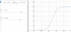
Logistic Curve

The logistic Curve with parameters.

A logistic function is S-shaped curve (or sigmoid curve) is a function with equation

$v(t)={\begin{cases}v(t)={\frac {L}{1+e^{-k(t-t_{0})}}}&&{\text{if }}t<t_{0}\\L&&{\text{if }}t\geq t_{0}\end{cases}}$

where $t_{0}$ is the $t$ value of the sigmoid's midpoint, $L$ is the curve's maximum value and $k$ is the curve's growth rate. See the Desmos graph.

The bumb function

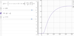
The Bumb Function.

There exists some well-known every-where differentiable functions, with a compact support. One example is

$v_{1}(t)={\begin{cases}1&&{\text{if }}-a<t<a\\e^{-{\frac {(|t|-a)^{2}}{4a^{2}-t^{2}}}}&&{\text{if }}a\leq |t|\\0&&{\text{if }}t>2a\end{cases}}$

with $v(t)=100v_{1}(t-180)$. This is an example of a $C^{\infty }$ with support in $a-r\leq t\leq a+r$. We are going to take half of the curve to be our velocity function. The graph is shown on Desmos page.

See more about the function at Math Stack Exchange, and the references therein.