Qiskit

Introduction

https://quantum-computing.ibm.com/

https://quantum-computing.ibm.com/challenges/fall-2020

https://quantum-computing.ibm.com/jupyter/user/IBMQuantumChallenge2020/week-1/ex_1a_en.ipynb

Theory

Installation

Installation https://qiskit.org/documentation/install.html

conda create -n qiskit python=3
conda activate qiskit
pip install qiskit _OR_ pip install qiskit[visualization]

Setting Up Qiskit

https://qiskit.org/textbook/ch-states/representing-qubit-states.html

qc = QuantumCircuit(1)  # Create a quantum circuit with one qubit
initial_state = [0,1]   # Define initial_state as |1>
qc.initialize(initial_state, 0) # Apply initialisation operation to the 0th qubit
qc.draw('text')  # Let's view our circuit (text drawing is required for the 'Initialize' gate due to a known bug in qiskit)
result = execute(qc,backend).result() # Do the simulation, returning the result
out_state = result.get_statevector()
print(out_state) # Display the output state vector

qc.measure_all()
qc.draw()
result = execute(qc,backend).result()
counts = result.get_counts()
plot_histogram(counts)

Take superposition as initial state

initial_state = [1/sqrt(2), 1j/sqrt(2)]  # Define state |q>

The Bloch Sphere

from qiskit_textbook.widgets import plot_bloch_vector_spherical
coords = [pi/2,0,1] # [Theta, Phi, Radius]
plot_bloch_vector_spherical(coords) # Bloch Vector with spherical coordinates

Qiskit allows measuring in the Z-basis, only.

Quantum Gates

Identity gate.

Pauli X gate. $\sigma _{x}=X={\begin{bmatrix}0&1\\1&0\end{bmatrix}}=|0\rangle \langle 1|+|1\rangle \langle 0|$

Pauli Y gate $\sigma _{y}=Y={\begin{bmatrix}0&-i\\i&0\end{bmatrix}}=-i|0\rangle \langle 1|+i|1\rangle \langle 0|$

Pauli Z gate $\sigma _{z}=Z={\begin{bmatrix}1&0\\0&-1\end{bmatrix}}=|0\rangle \langle 0|-|1\rangle \langle 1|$

Hadamard gate $H={\tfrac {1}{\sqrt {2}}}{\begin{bmatrix}1&1\\1&-1\end{bmatrix}}=|+\rangle \langle 0|+|-\rangle \langle 1|$

R gate $R_{\phi }={\begin{bmatrix}1&0\\0&e^{i\phi }\end{bmatrix}}$

S gate or ${\sqrt {Z}}$ gate $S={\begin{bmatrix}1&0\\0&e^{\frac {i\pi }{2}}\end{bmatrix}}$

T gate $T={\begin{bmatrix}1&0\\0&e^{\frac {i\pi }{4}}\end{bmatrix}}$

U1 gate: $U_{1}=U_{3}(0,0,\lambda )=U_{1}={\begin{bmatrix}1&0\\0&e^{i\lambda }\\\end{bmatrix}}$

U2 gate: $U_{2}=U_{3}({\tfrac {\pi }{2}},\phi ,\lambda )={\tfrac {1}{\sqrt {2}}}{\begin{bmatrix}1&-e^{i\lambda }\\e^{i\phi }&e^{i\lambda +i\phi }\end{bmatrix}}$

qc = QuantumCircuit(1)
qc.x(0)
#qc.y(0) # Y-gate on qubit 0
#qc.z(0) # Z-gate on qubit 0
#qc.rz(pi/4, 0)
#qc.s(0)   # Apply S-gate to qubit 0
#qc.sdg(0) # Apply Sdg-gate to qubit 0
qc.t(0)   # Apply T-gate to qubit 0
qc.tdg(0) # Apply Tdg-gate to qubit 0

qc.draw('mpl')
# Let's see the result
backend = Aer.get_backend('statevector_simulator')
out = execute(qc,backend).result().get_statevector()
plot_bloch_multivector(out)

Multiple Qubits

Eg. $X\otimes H={\begin{bmatrix}0&H\\H&0\end{bmatrix}}$.

backend = Aer.get_backend('unitary_simulator')
unitary = execute(qc,backend).result().get_unitary()
#
# In Jupyter Notebooks we can display this nicely using Latex.
# If not using Jupyter Notebooks you may need to remove the 
# array_to_latex function and use print(unitary) instead.
from qiskit_textbook.tools import array_to_latex
array_to_latex(unitary, pretext="\\text{Circuit = }\n")

CNOT gate as a pictoram.

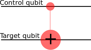
Eg. CNOT is a conditional gate that performs an X-gate on the second qubit, if the state of the first qubit (control) is $|1\rangle$. $CNOT={\begin{bmatrix}1&0&0&0\\0&0&0&1\\0&0&1&0\\0&1&0&0\\\end{bmatrix}}$. This matrix swaps the amplitudes of |01⟩ and |11⟩ in the statevector.

CNOT if a control qubit is on the superposition:

${\text{CNOT}}|{-}0\rangle =|{-}0\rangle$

${\text{CNOT}}|{-}1\rangle =-|{-}1\rangle$

${\text{CNOT}}|0{+}\rangle ={\tfrac {1}{\sqrt {2}}}(|00\rangle +|11\rangle )$, which is Bell State. Entanglement, but no-communication theorem.

${\text{CNOT}}|{+}{+}\rangle =|{+}{+}\rangle )$. Unchanged.

${\text{CNOT}}|{-}{+}\rangle ={\tfrac {1}{\sqrt {2}}}(|{-}0\rangle -|{-}1\rangle )=|{-}{-}\rangle$

${\text{CNOT}}|{+}{-}\rangle =$.

${\text{CNOT}}|{-}{-}\rangle ={\tfrac {1}{2}}(|00\rangle -|01\rangle -|10\rangle +|11\rangle )=|{-}{-}\rangle$. Affects the state of the control qubit, only.

qc = QuantumCircuit(2)
# Apply H-gate to the first:
qc.h(0)
# Apply a CNOT:
qc.cx(0,1)
qc.draw()
#
# Let's see the result:
backend = Aer.get_backend('statevector_simulator')
final_state = execute(qc,backend).result().get_statevector()
# Print the statevector neatly:
array_to_latex(final_state, pretext="\\text{Statevector = }")
#
results = execute(qc,backend).result().get_counts()
plot_histogram(results)

Any controlled quantum gate is ${\text{Controlled-U}}={\begin{bmatrix}I&0\\0&U\end{bmatrix}}$ and in Qiskit formalism is written in matrix as ${\text{Controlled-U}}={\begin{bmatrix}1&0&0&0\\0&u_{00}&0&u_{01}\\0&0&1&0\\0&u_{10}&0&u_{11}\\\end{bmatrix}}$

Controlled-Z. Because $HXH=Z$ and $HZH=X$ we can write

qc = QuantumCircuit(2)
# also a controlled-Z
qc.h(t)
qc.cx(c,t)
qc.h(t)
qc.draw()

Controlled-Y is

qc = QuantumCircuit(2)
# a controlled-Y
qc.sdg(t)
qc.cx(c,t)
qc.s(t)
qc.draw()

or Controlled-H is

</syntaxhighlight> qc = QuantumCircuit(2)

1. a controlled-H

qc.ry(pi/4,t) qc.cx(c,t) qc.ry(-pi/4,t) qc.draw() <syntaxhighlight>

Exercises

Week 1

Week 2

Week 3