Python and phyphox

Introduction

Phyphox XML and VIM

Activate the matchit.vim macro :runtime macros/matchit.vim and set the filetype :set filetype=html (or xml), and now % swaps between the tags.

The data is located in <data-containers> blocks and <container> tag contains the data of each measurements, but is in init tag, as shown below: <container size="0" init="1.009771156E1,1.012672424E1,1.004746246E1,1.009292603E1,1.024636555E1,1.024875832E1,1.015065289E1,1.007617569E1,1.012193871E1,1.011954594E1,9.999606133E0,9.978070259E0,1.0059426. Thus, we need to read the init part only.

Load the acceleration data

The simplest

import pandas as pd
df = pd.read_xml( filename )

does not work if the XML file is too large. Use lxml from etree instead:

from lxml import etree

def parse_lxml_large_xml(source, a):
    for event, elem in etree.iterparse(source, events=('end',)):
        if elem.tag == "container" and elem.text == a:
            #Split the string and convert to float
            A = elem.text
            B = elem.attrib
            BB = B.get('init').split(",")
            data = np.empty( (len( BB  ), 1 ) )
            for i, d in enumerate( BB ):
                data[i,0] = float(d)
            elem.clear()  # Free memory
    return data

and use it as

accX = parse_lxml_large_xml( "nousu_waw_tll_edited.phyphox", "accX" )
accY = parse_lxml_large_xml( "nousu_waw_tll_edited.phyphox", "accY" )
accZ = parse_lxml_large_xml( "nousu_waw_tll_edited.phyphox", "accZ" )
acc = parse_lxml_large_xml( "nousu_waw_tll_edited.phyphox", "acc" )
time = parse_lxml_large_xml( "nousu_waw_tll_edited.phyphox", "acc_time" )

A = np.column_stack( [time, accX, accY, accZ, acc]  )
df = pd.DataFrame( A, columns=['time', 'ax', 'ay', 'az', 'a'] )
df.set_index('time', inplace=True)

The last line changes the time column to be the index column, and the inplace keyword replaces that data directly into df variable.

We can load any other data similarly, too. Just change the the names in function calls.

Flights

1. Departure WAW-TLL: Plot the data

The raw total acceleration data with rolling mean

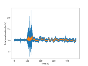
ax = df.a.plot()
ax = df.a.rolling(window=100).mean().plot(x='time')
ax.set_xlabel('Time [s]')
ax.set_ylabel("Total acceleration [m/s²]")
plt.show()

The rolling(window=100).mean() calculates the rolling mean with a window of width 100 to be plotted. The x='time' in parenthesis is not obligatory, as we already stated that the index is time. The two lines are to state the x and y labels better. The final line is to show the image.

The command

ax.legend(['All data', 'Rolling mean (100)'] )
plt.show()

will give the legend box. Note that the plt.show() need to be added here.

It is clearly shown that the something happens about at t=96 s; the acceleration changes from a bit over 10 to something else. However, even the smoothed data is rather difficult to visualize what happens.

1. Departure WAW-TLL: Check the Rolling mean

Different rolling window sizes

Adjust the separation between subfigures

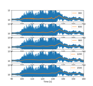
We need to check if the size of the window in the rolling gives different and perhaps easily interpreted figures.

fig = plt.figure()
for i in range(1,6):
    ax = fig.add_subplot(5,1,i)
    df.a.plot( label='_nolegend_' )
    df.a.rolling(window=i*300).mean().plot(x='time')
    ax.set_xlim([90,160])
    ax.set_ylim([9,15])
    ax.set_xlabel('Time [s]')
    ax.legend( [str(i*300) ] )
plt.show()

To loop many values, use for syntax. Set the limits to x and y axis to help visualize the data better. Also depict in the legend what is the window size. The legend of the original (blue) line is not shown, because its label is stated _nolegend.

The xlabels are are partly hidden below the images, and there is some empty space between the subfigure panels. We could remove those, but the zooming becomes difficult as the different subfigures zoom at different rates. but for printing purposes that would be good option.

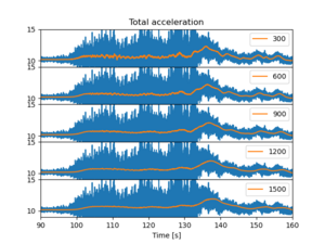
Thus add the following commands to be end of the for loop:

    if i<5:
        ax.set_xticks([])
    if i==1:
        ax.set_title('Total acceleration')
plt.subplots_adjust(hspace=0.)

Don't forget to the plt.show() command.

We note that though the rolling mean is about similar in all the cases, the larger is better. Next we will study the acceleration in different axes.

1. Departure WAW-TLL: Analyze the acceleration along axes

The acceleration axes are following:

• a_x left/ right
• a_y forward/ backward
• a_z up/ down

<syntaxhighlight lang="python"> <syntaxhighlight>

<syntaxhighlight lang="python"> <syntaxhighlight>