Yolo Pose Estimation and Skeleton: Difference between revisions
| (19 intermediate revisions by the same user not shown) | |||
| Line 91: | Line 91: | ||
Use cv2 to plot the image. This cv2 plotting will be used in the next part. | Use '''cv2''' to plot the image. This cv2 plotting will be used in the next part. | ||
<syntaxhighlight lang="python"> | <syntaxhighlight lang="python"> | ||
image = cv2.imread(filename) | image = cv2.imread(filename) | ||
| Line 100: | Line 100: | ||
cv2.waitKey(0) | cv2.waitKey(0) | ||
cv2.destroyAllWindows() | cv2.destroyAllWindows() | ||
</syntaxhighlight> | |||
Use '''Pillow''' to plot the image. This cv2 plotting will be used in the next part. | |||
<syntaxhighlight lang="python"> | |||
import numpy as np | |||
xy_knee = results[0].keypoints.xy[0][14] | |||
xyknee = np.asarray( xy_knee.cpu() ).astype(np.int64) | |||
image = Image.open(filename).convert('RGBA') | |||
bone_femur = Image.open('femur_left.png').convert('RGBA') | |||
Image.Image.paste(image, bone_femur, tuple(xyhip), bone_femur ) #Use the mask | |||
</syntaxhighlight> | </syntaxhighlight> | ||
| Line 106: | Line 121: | ||
A CUDA:0 tensor is a tensor that is stored on a GPU, and thus isn't accessible to the CPU. To have it in Numpy, use: | A CUDA:0 tensor is a tensor that is stored on a GPU, and thus isn't accessible to the CPU. To have it in Numpy, use: | ||
# Copy the data from the GPU to the CPU: `torch.cuda.to_cpu()`. | # Copy the data from the GPU to the CPU: `torch.cuda.to_cpu()`. | ||
# Reorder the data (from a column-major format to a row-major): `numpy.transpose()`. | # Reorder the data (from a column-major format to a row-major): `numpy.transpose()`. Not needed in this simple 1d example. | ||
# Convert the data to NumPy: `numpy.asarray()`. | # Convert the data to NumPy: `numpy.asarray()`, and convert to integer. | ||
<syntaxhighlight lang="python"> | |||
xy_hip =results[0].keypoints.xy[0][12] | |||
cpu_xyhip = np.asarray( xy_hip.cpu() ).astype(np.int64) #Copy and convert; | |||
</syntaxhighlight> | |||
=== Draw joints and an arrow in between === | |||
<gallery> | |||
Yolo joints.PNG|thumb|Circles represent the joints. The position is adjusted to the middle of the circle. | |||
Yolo joints arrow.PNG|thumb|The arrow in between the joints. The position is not adjusted to exactly correct place as it might not be important in case of the bones. | |||
</gallery> | |||
Make a circle.png and draw that on the image. The insertion point is the upper left corner, so we need to adjust it a bit so that the joint is in the middle of circle. | |||
<syntaxhighlight lang="python"> | |||
image = Image.open(filename).convert('RGBA') | |||
joint = Image.open('circle.png').convert('RGBA') | |||
joint_size = joint.size | |||
for i in range(17): | |||
p=results[0].keypoints.xy[0][i] | |||
p = np.asarray( p.cpu() ).astype(np.int64) #Copy and convert; | |||
p[0], p[1] = p[0] - joint_size[0]/2, p[1] - joint_size[1]/2 | |||
Image.Image.paste(image, joint, tuple(p), joint ) #Use the mask | |||
image.show() | |||
</syntaxhighlight> | |||
Add the arrow.png in between the joints. | |||
<syntaxhighlight lang="python"> | |||
arrow = Image.open('arrow.png').convert('RGBA') | |||
arrow_size = arrow.size | |||
print( arrow_size ) | |||
#Add the joints | |||
for i in [12,14]: | |||
p=results[0].keypoints.xy[0][i] | |||
p = np.asarray( p.cpu() ).astype(np.int64) #Copy and convert; | |||
p[0], p[1] = p[0] - joint_size[0]/2, p[1] - joint_size[1]/2 | |||
Image.Image.paste(image, joint, tuple(p), joint ) #Use the mask | |||
xy_knee = results[0].keypoints.xy[0][14] | |||
xyknee = np.asarray( xy_knee.cpu() ).astype(np.int64) | |||
xy_hip =results[0].keypoints.xy[0][12] | |||
xyhip = np.asarray( xy_hip.cpu() ).astype(np.int64) #Copy and convert; | |||
d = xyknee- xyhip | |||
dist = np.linalg.norm(d) | |||
angle = 90 - np.arctan2( d[1], d[0] )*180/np.pi | |||
print( angle, dist ) | |||
bone_femur = Image.open('arrow.png').convert('RGBA').resize( (int(dist*arrow_size[0]/arrow_size[1]), int(dist) )).rotate(angle, Image.NEAREST, expand=1) | |||
Image.Image.paste(image, bone_femur, tuple(xyhip), bone_femur ) #Use the mask | |||
</syntaxhighlight> | |||
=== Pose to skeleton === | === Pose to skeleton === | ||
| Line 114: | Line 188: | ||
* 12 (left hip) and 14 (left knee) or | * 12 (left hip) and 14 (left knee) or | ||
* 13 (right hip) and 15 (right knee) | * 13 (right hip) and 15 (right knee) | ||
First, plot a line between the joints: | |||
<syntaxhighlight lang="python"> | |||
xy_knee = results[0].keypoints.xy[0][14] | |||
xyknee = np.asarray( xy_knee.cpu() ).astype(np.int64) | |||
xy_hip =results[0].keypoints.xy[0][12] | |||
xyhip = np.asarray( xy_hip.cpu() ).astype(np.int64) #Copy and convert; | |||
cv2.line( image, xyhip , xyknee, (0,250,0), 9) | |||
</syntaxhighlight> | |||
Then, get the angle and insert the image of the bone instead. | |||
=== Combine/ blend images === | |||
Pillow, cv2, Scikit-image. | |||
* https://stackoverflow.com/questions/55795755/how-to-add-an-image-over-another-image-using-x-y-coordinates | |||
PIL | |||
* <code>Image.Image.paste(im1, im2, (50, 125))</code> | |||
* <code>im1 = im1.rotate(90, PIL.Image.NEAREST, expand = 1)</code> | |||
PIL and cv2 | |||
<syntaxhighlight lang="python"> | |||
pil_im = Image.open("image.jpg") | |||
cv_im = cv2.cvtColor(np.array(pil_im), cv2.COLOR_RGB2BGR) | |||
# Apply OpenCV operations | |||
edges = cv2.Canny(cv_im, 100, 200) | |||
# Convert back to PIL and display | |||
pil_edges = Image.fromarray(edges) | |||
pil_edges.show() | |||
</syntaxhighlight> | |||
=== === | === === | ||
== Images == | == Images == | ||
=== Use the laptop camera === | |||
Scale the image height to 400 px and width such that the center of bone is in the middle of the image. | |||
Show video only | |||
<syntaxhighlight lang="python"> | |||
import cv2 | |||
cap = cv2.VideoCapture(0) | |||
while True: | |||
ret,img=cap.read() | |||
cv2.imshow('Video', img) | |||
if(cv2.waitKey(10) & 0xFF == ord('b')): | |||
break | |||
</syntaxhighlight> | |||
Show video with yolo | |||
<syntaxhighlight lang="python"> | |||
import cv2 | |||
cap = cv2.VideoCapture(0) | |||
while True: | |||
ret,img=cap.read() | |||
results = yolo.track(img, stream=True) | |||
print( results ) | |||
if(cv2.waitKey(10) & 0xFF == ord('b')): | |||
break | |||
</syntaxhighlight> | |||
=== 2 === | |||
=== 3 === | |||
== Video == | == Video == | ||
| Line 125: | Line 271: | ||
* https://medium.com/@staytechrich/human-pose-estimation-with-yolov11-96932a5d7159 | * https://medium.com/@staytechrich/human-pose-estimation-with-yolov11-96932a5d7159 | ||
* https://www.labellerr.com/blog/how-to-perform-yolos-various-task/ | * https://www.labellerr.com/blog/how-to-perform-yolos-various-task/ | ||
* https://www.bomberbot.com/python/mastering-pythons-pil-image-show-method-a-deep-dive-for-developers/ | |||
Latest revision as of 15:31, 14 October 2025
Introduction
Make a pose estimator and use it to make a moving skeleton.
Use Yolo from Ultralytics.
- Python 3.7+
- Yolo v11
- A CUDA-enabled GPU (optional but recommended for faster inference).
pip install ultralytics opencv-python numpy
Yolo
There are 17 keypoints. YOLOv11’s pose model outputs:
- (x, y) coordinates for each keypoint and
- confidence scores indicating the model’s certainty in each keypoint’s position.
Image detection
-
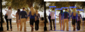
AN image before and after the code.
from ultralytics import YOLO
import matplotlib.pyplot as plt
import cv2
#from PIL import Image

model = YOLO("yolo11n-pose.pt")  # n, s, m, l, x versions available

results = model.predict(source="sample_image.jpg")

plt.figure(figsize=(10, 10))
plt.title('YOLOv11 Pose Results')
plt.axis('off')
plt.imshow(cv2.cvtColor(results[0].plot(), cv2.COLOR_BGR2RGB))
The results list includes results[0].keypoints.xy, results[0].keypoints.xyn and results[0].keypoints.conf data. Printing that gives some general information about what is found and how fast, and a tensor vector which includes the position data.
image 1/1 /home/mol/Documents/python/skeletor/people2.jpg: 512x640 5 persons, 26.0ms
Speed: 1.4ms preprocess, 26.0ms inference, 38.0ms postprocess per image at shape (1, 3, 512, 640)
tensor([[[1608.5103,  516.1241],
         [1600.1213,  497.7412],
         [1613.1257,  497.1426],
         [1568.5618,  506.6950],
         [1648.6650,  505.3312],
         [1556.0571,  614.9849],
         [1692.7899,  615.2242],
         [1540.9780,  763.7505],
         [1755.1765,  773.1780],
         [1548.3131,  886.3889],
         [1795.6322,  892.2405],
         [1588.8513,  896.8289],
         [1680.1824,  896.3278],
         [1574.6792, 1117.8225],
         [1675.2017, 1118.2271],
         [1589.6167, 1317.0865],
         [1671.6086, 1320.7114]],

        [[1097.3536,  432.4247],
         [1086.8494,  405.5817],
         [1092.0603,  402.9798],
         [ 987.7101,  409.1143],
         [1076.7693,  412.7003],
         [ 924.9458,  531.9528],
         [1117.5946,  533.4085],
         [ 875.2901,  720.3015],
         [1186.5740,  715.3069],
         [ 862.7459,  861.0502],
         [1189.9052,  849.3643],
         [ 957.1283,  837.9849],
         [1090.0930,  841.1834],
         [ 920.7561, 1110.6389],
         [1099.1434, 1116.8433],
         [ 925.5239, 1367.9281],
         [1102.7339, 1381.9753]],
To print the coordinates of keypoints, use
for r in results[0].keypoints.xy:
    print(r)
Use cv2 to plot the image. This cv2 plotting will be used in the next part.
image = cv2.imread(filename)

cv2.namedWindow("image", cv2.WINDOW_KEEPRATIO)
cv2.imshow("image", image)
cv2.resizeWindow("image", 600, 600)
cv2.waitKey(0)
cv2.destroyAllWindows()
Use Pillow to plot the image. This cv2 plotting will be used in the next part.
import numpy as np

xy_knee = results[0].keypoints.xy[0][14]
xyknee = np.asarray( xy_knee.cpu() ).astype(np.int64)

image = Image.open(filename).convert('RGBA')
bone_femur = Image.open('femur_left.png').convert('RGBA')

Image.Image.paste(image, bone_femur, tuple(xyhip), bone_femur )  #Use the mask
CUDA:0 problem
A CUDA:0 tensor is a tensor that is stored on a GPU, and thus isn't accessible to the CPU. To have it in Numpy, use:
- Copy the data from the GPU to the CPU: `torch.cuda.to_cpu()`.
- Reorder the data (from a column-major format to a row-major): `numpy.transpose()`. Not needed in this simple 1d example.
- Convert the data to NumPy: `numpy.asarray()`, and convert to integer.
xy_hip =results[0].keypoints.xy[0][12]
cpu_xyhip = np.asarray( xy_hip.cpu() ).astype(np.int64) #Copy and convert;
Draw joints and an arrow in between
-
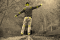
Circles represent the joints. The position is adjusted to the middle of the circle.
-
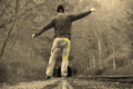
The arrow in between the joints. The position is not adjusted to exactly correct place as it might not be important in case of the bones.

Make a circle.png and draw that on the image. The insertion point is the upper left corner, so we need to adjust it a bit so that the joint is in the middle of circle.
image = Image.open(filename).convert('RGBA')
joint = Image.open('circle.png').convert('RGBA')
joint_size = joint.size

for i in range(17):
    p=results[0].keypoints.xy[0][i]
    p = np.asarray( p.cpu() ).astype(np.int64) #Copy and convert;
    p[0], p[1] = p[0] - joint_size[0]/2, p[1] - joint_size[1]/2

    Image.Image.paste(image, joint, tuple(p), joint )  #Use the mask

image.show()
Add the arrow.png in between the joints.
arrow = Image.open('arrow.png').convert('RGBA')
arrow_size = arrow.size
print( arrow_size )

#Add the joints
for i in [12,14]:
    p=results[0].keypoints.xy[0][i]
    p = np.asarray( p.cpu() ).astype(np.int64) #Copy and convert;
    p[0], p[1] = p[0] - joint_size[0]/2,  p[1] - joint_size[1]/2

    Image.Image.paste(image, joint, tuple(p), joint )  #Use the mask


xy_knee = results[0].keypoints.xy[0][14]
xyknee = np.asarray( xy_knee.cpu() ).astype(np.int64)
xy_hip =results[0].keypoints.xy[0][12]
xyhip = np.asarray( xy_hip.cpu() ).astype(np.int64) #Copy and convert;
d = xyknee- xyhip
dist = np.linalg.norm(d)
angle = 90 - np.arctan2( d[1], d[0] )*180/np.pi
print( angle, dist )
bone_femur = Image.open('arrow.png').convert('RGBA').resize( (int(dist*arrow_size[0]/arrow_size[1]), int(dist) )).rotate(angle, Image.NEAREST, expand=1)

Image.Image.paste(image, bone_femur, tuple(xyhip), bone_femur )  #Use the mask
Pose to skeleton
The keypoint coordinates need to be converted to bones; as an example, femur is located between
- 12 (left hip) and 14 (left knee) or
- 13 (right hip) and 15 (right knee)
First, plot a line between the joints:
xy_knee = results[0].keypoints.xy[0][14]
xyknee = np.asarray( xy_knee.cpu() ).astype(np.int64)

xy_hip =results[0].keypoints.xy[0][12]
xyhip = np.asarray( xy_hip.cpu() ).astype(np.int64) #Copy and convert;

cv2.line( image, xyhip , xyknee, (0,250,0), 9)
Then, get the angle and insert the image of the bone instead.
Combine/ blend images
Pillow, cv2, Scikit-image.
PIL
Image.Image.paste(im1, im2, (50, 125))im1 = im1.rotate(90, PIL.Image.NEAREST, expand = 1)
PIL and cv2
pil_im = Image.open("image.jpg")
cv_im = cv2.cvtColor(np.array(pil_im), cv2.COLOR_RGB2BGR)

# Apply OpenCV operations
edges = cv2.Canny(cv_im, 100, 200)

# Convert back to PIL and display
pil_edges = Image.fromarray(edges)
pil_edges.show()
Images
Use the laptop camera
Scale the image height to 400 px and width such that the center of bone is in the middle of the image.
Show video only
import cv2
cap = cv2.VideoCapture(0)

while True:
    ret,img=cap.read()
    cv2.imshow('Video', img)
    if(cv2.waitKey(10) & 0xFF == ord('b')):
        break
Show video with yolo
import cv2
cap = cv2.VideoCapture(0)

while True:
    ret,img=cap.read()
    results = yolo.track(img, stream=True)
    print( results )

    if(cv2.waitKey(10) & 0xFF == ord('b')):
        break