Lidar data visualization: Difference between revisions
(→Theory) |
No edit summary |
||
| (24 intermediate revisions by the same user not shown) | |||
| Line 10: | Line 10: | ||
[https://en.wikipedia.org/wiki/LAS_file_format LAS@Wikipedia] | [https://en.wikipedia.org/wiki/LAS_file_format LAS@Wikipedia] | ||
[https://3dprinting.stackexchange.com/questions/882/how-to-print-lidar-file-format-las#884 how to print lidar file format las] | [https://3dprinting.stackexchange.com/questions/882/how-to-print-lidar-file-format-las#884 how to print lidar file format las] | ||
a) Headers. | |||
b) VLR: Variable Length Record. Include 1) header and 2) payload. | |||
c) Point records. Different point formats 0-10. | |||
=== LAS in Python === | === LAS in Python === | ||
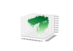
[[File:LasImagePython.png|thumb|To check if the data points are there]] | |||
[[https://github.com/tmontaigu/pylas PyLAS Github]] | [[https://github.com/tmontaigu/pylas PyLAS Github]] | ||
| Line 18: | Line 26: | ||
[[https://github.com/grantbrown/laspy Laspy Github]] [[https://pypi.org/project/laspy/ LasPy]] | [[https://github.com/grantbrown/laspy Laspy Github]] [[https://pypi.org/project/laspy/ LasPy]] | ||
[[https://jblindsay.github.io/ghrg/WhiteboxTools/interpolate_lidar.html]] | |||
<syntaxhighlight lang="python"> | |||
import numpy as np | |||
import pylas | |||
las = pylas.read( fname ) | |||
#np.all(las.user_data == las['user_data']) | |||
point_format = las.point_format | |||
print( point_format ) | |||
print( point_format.id ) | |||
print( list(point_format.dimension_names) ) | |||
from mpl_toolkits import mplot3d | |||
import matplotlib.pyplot as plt | |||
fig = plt.figure() | |||
ax = plt.axes(projection='3d') | |||
N=5000 | |||
ax.scatter3D(las.X[:N], las.Y[:N], las.Z[:N], c=las.Z[:N], cmap='Greens'); | |||
</syntaxhighlight> | |||
=== Lidar Cloud Data to Blender Mesh using Opend3D=== | |||
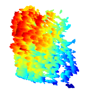
[[File:Open3D las datapoints.png|thumb|The full dataset rendered in OpenGL.]] | |||
Blender needs mesh, also nodes, faces and vertices. Thus, the data cloud need to be converted to mesh data. We use the Rolling Ball algorithm of Open3d package. | |||
Read the data and convert it to a suitable format for Open3D. Also visualize it: | |||
<syntaxhighlight lang="python"> | |||
fname = '20150608_it-ren_nadir_densified_point_cloud_merged.las' | |||
import open3d as o3d | |||
import pylas | |||
las = pylas.read( fname ) | |||
print('Points from data:', len(las.points)) | |||
N=100000 | |||
N=25797964 | |||
X = np.transpose( [las.X[:N], las.Y[:N], las.Z[:N]] ) | |||
cloud = o3d.geometry.PointCloud() | |||
cloud.points = o3d.utility.Vector3dVector(X) | |||
cloud.estimate_normals() | |||
#Mesh: Poisson Reconstruction | |||
mesh_poisson = o3d.geometry.TriangleMesh.create_from_point_cloud_poisson( | |||
cloud, depth=10, width=0, scale=1.1, linear_fit=False)[0] | |||
o3d.io.write_triangle_mesh("mesh_poisson_10.ply", mesh_poisson ) | |||
</syntaxhighlight> | |||
It might be possible to generate the mesh using the rolling ball algorithm; however, the capacity of my computer is not sufficient. Thus the following is not tested: | |||
<syntaxhighlight lang="python"> | |||
#Mesh: The rolling ball algorithm | |||
# estimate radius for rolling ball | |||
distances = cloud.compute_nearest_neighbor_distance() | |||
avg_dist = np.mean(distances) | |||
radius = 1.5 * avg_dist | |||
radius = 5*avg_dist | |||
mesh = o3d.geometry.TriangleMesh.create_from_point_cloud_ball_pivoting( | |||
cloud, | |||
o3d.utility.DoubleVector([radius, radius * 2])) | |||
</syntaxhighlight> | |||
The mesh is located according to the GPS coordinates, and the size is similar. Thus, the mesh need to be translated and scaled before importing to the Blender. | |||
<syntaxhighlight lang="python"> | |||
import numpy as np | |||
import pylas | |||
import open3d as o3d | |||
mesh = o3d.io.read_triangle_mesh("mesh_poisson_9.ply" ) | |||
print( mesh ) | |||
print(np.asarray(mesh.vertices)) | |||
X = np.asarray(mesh.vertices)[0] | |||
print(X) | |||
# | |||
# | |||
# | |||
import copy | |||
mesh_mv = copy.deepcopy(mesh).translate([0,0,0], relative=False) | |||
mesh_mv.scale(0.00001, center=mesh_mv.get_center()) | |||
print(f'Center of mesh: {mesh.get_center()}') | |||
print(f'Center of mesh_mv: {mesh_mv.get_center()}') | |||
o3d.io.write_triangle_mesh("mesh_poisson_9_ori.ply", mesh_mv ) | |||
</syntaxhighlight> | |||
Visualize the ply mesh. | |||
<syntaxhighlight lang="python"> | |||
port numpy as np | |||
import pylas | |||
import open3d as o3d | |||
#Poisson Reconstruction | |||
mesh = o3d.io.read_triangle_mesh("mesh_poisson_10.ply" ) | |||
mesh.compute_vertex_normals() | |||
mesh.paint_uniform_color([1, 0.706, 0]) | |||
o3d.visualization.draw_geometries([mesh]) | |||
print( mesh ) | |||
print(np.asarray(mesh.vertices)) | |||
</syntaxhighlight> | |||
[https://stackoverflow.com/questions/56965268/how-do-i-convert-a-3d-point-cloud-ply-into-a-mesh-with-faces-and-vertices how do i convert a 3d point cloud ply into a mesh with faces and vertices] | |||
[https://assettocorsamods.net/threads/lidar-point-cloud-to-mesh-tutorial.422/ Cloud to Mesh Tutorial] | |||
[https://jblindsay.github.io/ghrg/WhiteboxTools/interpolate_lidar.html Interpolate lidar ] | |||
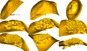
=== Poisson Depth === | |||
The depth in Poisson reconstruction has an effect. | |||
[[File:PoissonDepths.png|thumb|The depth in Poisson.]] | |||
=== Render data in Blender === | |||
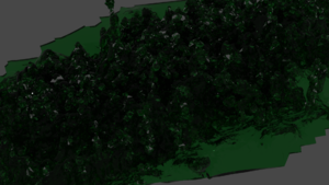
[[File:BlenderRenderedGlassForest.png|thumb|The dark and glassy forest. ]] | |||
The translated and scaled ply data can be imported to blender. After importing I edited the mesh structure and removed the overlap bulk mesh, changed the material to glassy (Principled BSDF and Transomission to 1). I added a modifier Solidify, and changed the color. Use the cycles renderer and changes the Render Samples to 300, perhaps. | |||
https://www.youtube.com/watch?v=643CAA5Zh_8 | |||
[https://re.je/blog/2014-04-11-rendering-point-clouds-in-blender/ Rendering cloud data in Blender] | |||
[[Category:Blender]] | |||
[[Category:Python]] | |||
[[Category:LiDar]] | |||
Latest revision as of 19:23, 11 February 2021
Introduction
Use Lidar data, post analyze it with Python/ Pandas? and use Blender to visualize it.
Theory
The free Lidar data set are available e.g. at Opentopography.org. We use both, the Tif data and LAS data of IT-Ren, Fluxnet site
LAS File Format
LAS@Wikipedia how to print lidar file format las
a) Headers.
b) VLR: Variable Length Record. Include 1) header and 2) payload.
c) Point records. Different point formats 0-10.
LAS in Python

[Laspy Github] [LasPy]
import numpy as np
import pylas

las = pylas.read( fname )
#np.all(las.user_data == las['user_data'])

point_format = las.point_format
print( point_format )
print( point_format.id )
print( list(point_format.dimension_names) )

from mpl_toolkits import mplot3d
import matplotlib.pyplot as plt
fig = plt.figure()
ax = plt.axes(projection='3d')

N=5000
ax.scatter3D(las.X[:N], las.Y[:N], las.Z[:N], c=las.Z[:N], cmap='Greens');
Lidar Cloud Data to Blender Mesh using Opend3D

Blender needs mesh, also nodes, faces and vertices. Thus, the data cloud need to be converted to mesh data. We use the Rolling Ball algorithm of Open3d package.
Read the data and convert it to a suitable format for Open3D. Also visualize it:
fname =  '20150608_it-ren_nadir_densified_point_cloud_merged.las'

import open3d as o3d
import pylas
las = pylas.read( fname )
print('Points from data:', len(las.points))

N=100000
N=25797964
X = np.transpose( [las.X[:N], las.Y[:N], las.Z[:N]] )
cloud = o3d.geometry.PointCloud()
cloud.points = o3d.utility.Vector3dVector(X)

cloud.estimate_normals()

#Mesh: Poisson Reconstruction
mesh_poisson = o3d.geometry.TriangleMesh.create_from_point_cloud_poisson(
        cloud, depth=10, width=0, scale=1.1, linear_fit=False)[0]

o3d.io.write_triangle_mesh("mesh_poisson_10.ply", mesh_poisson )
It might be possible to generate the mesh using the rolling ball algorithm; however, the capacity of my computer is not sufficient. Thus the following is not tested:
#Mesh: The rolling ball algorithm
# estimate radius for rolling ball
distances = cloud.compute_nearest_neighbor_distance()
avg_dist = np.mean(distances)
radius = 1.5 * avg_dist
radius = 5*avg_dist

mesh = o3d.geometry.TriangleMesh.create_from_point_cloud_ball_pivoting(
           cloud,
           o3d.utility.DoubleVector([radius, radius * 2]))
The mesh is located according to the GPS coordinates, and the size is similar. Thus, the mesh need to be translated and scaled before importing to the Blender.
import numpy as np
import pylas
import open3d as o3d

mesh = o3d.io.read_triangle_mesh("mesh_poisson_9.ply" )

print( mesh )
print(np.asarray(mesh.vertices))
X = np.asarray(mesh.vertices)[0]
print(X)
#
#
#
import copy
mesh_mv = copy.deepcopy(mesh).translate([0,0,0], relative=False)
mesh_mv.scale(0.00001, center=mesh_mv.get_center())

print(f'Center of mesh: {mesh.get_center()}')
print(f'Center of mesh_mv: {mesh_mv.get_center()}')

o3d.io.write_triangle_mesh("mesh_poisson_9_ori.ply", mesh_mv )
Visualize the ply mesh.
port numpy as np
import pylas

import open3d as o3d

#Poisson Reconstruction
mesh = o3d.io.read_triangle_mesh("mesh_poisson_10.ply" )
mesh.compute_vertex_normals()
mesh.paint_uniform_color([1, 0.706, 0])

o3d.visualization.draw_geometries([mesh])

print( mesh )
print(np.asarray(mesh.vertices))
how do i convert a 3d point cloud ply into a mesh with faces and vertices
Poisson Depth
The depth in Poisson reconstruction has an effect.

Render data in Blender

The translated and scaled ply data can be imported to blender. After importing I edited the mesh structure and removed the overlap bulk mesh, changed the material to glassy (Principled BSDF and Transomission to 1). I added a modifier Solidify, and changed the color. Use the cycles renderer and changes the Render Samples to 300, perhaps.