OSM rivers to one main branch Python: Difference between revisions
| (20 intermediate revisions by the same user not shown) | |||
| Line 4: | Line 4: | ||
Finland map.png|The river map of Finland. The main river is plotted using larger linewidth than the tertiarys. | Finland map.png|The river map of Finland. The main river is plotted using larger linewidth than the tertiarys. | ||
Rivers of finland.png|1. The first plot of all the rivers without modifications. | Rivers of finland.png|1. The first plot of all the rivers without modifications. | ||
Kemijoki tributaries.png|2. The main branch and tributaries. | |||
</gallery> | </gallery> | ||
| Line 12: | Line 13: | ||
# There are many rivers haring the same name | # There are many rivers haring the same name | ||
# The shp data breaks | # The shp data breaks | ||
# There are cycles (loops) and branches | # There are cycles (loops) and tributaries (branches) | ||
== 1. Plot and check == | == 1. Plot and check == | ||
The analysis of different coordinate systems is shown elsewhere. | The analysis of different coordinate systems is shown elsewhere. | ||
=== Plot all Waterways === | |||
<syntaxhighlight lang="Python"> | <syntaxhighlight lang="Python"> | ||
| Line 46: | Line 49: | ||
plt.show() | plt.show() | ||
</syntaxhighlight > | </syntaxhighlight > | ||
=== The shp datafile === | |||
General format | |||
*.shp = shapes | |||
*.dbf = table (like a spreadsheet with headers) | |||
*.prj = map projection | |||
<syntaxhighlight lang="python> | |||
print(rivers.head()) | |||
osm_id ... geometry | |||
0 4251428 ... LINESTRING (384623.065 6671261.378, 384613.062... | |||
1 4336744 ... LINESTRING (424219.382 6758572.023, 424231.281... | |||
2 4418854 ... LINESTRING (271969.063 6961997.189, 272511.243... | |||
3 4418989 ... LINESTRING (263355.182 6994559.516, 263029.852... | |||
4 4494437 ... LINESTRING (235473.685 6716109.64, 235468.154 ... | |||
</syntaxhighlight> | |||
<syntaxhighlight lang="python> | |||
print(rivers.columns) | |||
Index(['osm_id', 'code', 'fclass', 'width', 'name', 'geometry'], dtype='object') | |||
</syntaxhighlight> | |||
<syntaxhighlight lang="python> | |||
print( rivers.info() ) | |||
<class 'geopandas.geodataframe.GeoDataFrame'> | |||
RangeIndex: 127503 entries, 0 to 127502 | |||
Data columns (total 6 columns): | |||
# Column Non-Null Count Dtype | |||
--- ------ -------------- ----- | |||
0 osm_id 127503 non-null object | |||
1 code 127503 non-null int32 | |||
2 fclass 127503 non-null object | |||
3 width 127503 non-null int32 | |||
4 name 26074 non-null object | |||
5 geometry 127503 non-null geometry | |||
dtypes: geometry(1), int32(2), object(3) | |||
memory usage: 4.9+ MB | |||
None | |||
</syntaxhighlight> | |||
<syntaxhighlight lang="python> | |||
print( river( ['fclass'].value_counts() ) | |||
fclass | |||
stream 104937 | |||
river 12776 | |||
drain 9186 | |||
canal 604 | |||
Name: count, dtype: int64 | |||
</syntaxhighlight> | |||
<syntaxhighlight lang="python> | |||
print(rivers.geometry) | |||
0 LINESTRING (384623.065 6671261.378, 384613.062... | |||
1 LINESTRING (424219.382 6758572.023, 424231.281... | |||
2 LINESTRING (271969.063 6961997.189, 272511.243... | |||
3 LINESTRING (263355.182 6994559.516, 263029.852... | |||
4 LINESTRING (235473.685 6716109.64, 235468.154 ... | |||
... | |||
127498 LINESTRING (193860.594 6771306.041, 193862.48 ... | |||
127499 LINESTRING (193500.06 6770531.712, 193481.661 ... | |||
127500 LINESTRING (267357.405 6823421.996, 267348.152... | |||
127501 LINESTRING (266604.152 6824271.814, 266614.528... | |||
127502 LINESTRING (543881.124 6893248.187, 543974.428... | |||
Name: geometry, Length: 127503, dtype: geometry | |||
</syntaxhighlight> | |||
<syntaxhighlight lang="python> | |||
print(rivers.describe(include='all')) | |||
osm_id ... geometry | |||
count 127503 ... 127503 | |||
unique 127503 ... 127502 | |||
top 4251428 ... LINESTRING (388682.74185180914 6718165.8999426... | |||
freq 1 ... 2 | |||
mean NaN ... NaN | |||
std NaN ... NaN | |||
min NaN ... NaN | |||
25% NaN ... NaN | |||
50% NaN ... NaN | |||
75% NaN ... NaN | |||
max NaN ... NaN | |||
[11 rows x 6 columns] | |||
</syntaxhighlight> | |||
<syntaxhighlight lang="python> | |||
gdf['name'].dropna().head(20) | |||
0 Ruoholahdenkanava | |||
1 Porvoonjoki | |||
2 Kyrönjoki | |||
3 Kyrönjoki | |||
4 Raisionjoki | |||
5 Riipinluoma | |||
6 Tjäck Ã¥ | |||
7 Kyrönjoki | |||
8 Kyrönjoki | |||
9 Kyro Älv | |||
10 Jalasjoki | |||
11 Kupparinoja | |||
12 Harjunjoki | |||
13 Jyräänjoki | |||
15 Hirvenjoki | |||
16 Takajoki | |||
18 Juotjoki | |||
21 Luhtaanmäenjoki | |||
22 Kostianvirta | |||
23 Ahlaistenjoki | |||
Name: name, dtype: object | |||
</syntaxhighlight> | |||
== 2. Plot Kemijoki and tributaries == | == 2. Plot Kemijoki and tributaries == | ||
<gallery> | |||
Kemijoki 2b border1.png|The effect of buffer | |||
Kemijoki 2b buffer2.png|Larger buffer | |||
Kemijoki 2b clipped10.png|Clipped with 10 km buffer | |||
Kemijoki 2b clipped20.png|Clipped with 20 km buffer | |||
Kemijoki 2b clipped40.png|Clipped with 40 km buffer | |||
Kemijoki 2b clipped80.png|Clipped with 80 km buffer | |||
Kemijoki 2b maingeometryUnaryUnion.png|The unary union of the main geometry | |||
Kemijoki 2b maingeometryUnaryUnionConnected.png|Connected, intersections | |||
Kemijoki 2b touching1.png|Touching 1. Buffer 80 km. | |||
Kemijoki 2b touching2.png|Touching 2. Buffer 80 km. | |||
Kemijoki 2b touching3.png|Touching 3. Buffer 80 km. | |||
Kemijoki 2b touching4.png|Touching 4. Buffer 80 km. | |||
Kemijoki 2b touching5.png|Touching 5. Buffer 80 km. | |||
Kemijoki 2b touching10.png|Touching 10. Buffer 80 km. | |||
Kemijoki 2b touching20.png|Touching 10. Buffer 80 km. | |||
</gallery> | |||
The beginning (loading the river data files and converting) is the same as before. | |||
<syntaxhighlight lang="Python"> | <syntaxhighlight lang="Python"> | ||
kemijoki = rivers[rivers["name"] == "Kemijoki"] | |||
buffer = kemijoki.buffer(50000) # 20 km buffer around the Kemijoko | |||
buffer_gdf = gpd.GeoDataFrame(geometry=buffer, crs=rivers.crs) | |||
kemijoki_rivers = gpd.clip(rivers, buffer_gdf) | |||
#Find the connected parts | |||
main_geom = unary_union(kemijoki.geometry) | |||
connected = kemijoki_rivers[kemijoki_rivers.geometry.intersects(main_geom)] | |||
current = main_geom | |||
for i in range(5): # increase if needed | |||
touching = kemijoki_rivers[kemijoki_rivers.geometry.intersects(current)] | |||
current = unary_union(touching.geometry) | |||
final_rivers = kemijoki_rivers[kemijoki_rivers.geometry.intersects(current)] | |||
# Plot it | |||
fig, ax = plt.subplots(figsize=(6, 10)) | |||
finland.plot(ax=ax, color="#f0f0f0", edgecolor="gray") | |||
final_rivers.plot(ax=ax, color="blue", linewidth=0.4) | |||
kemijoki.plot(ax=ax, color="darkblue", linewidth=1.5) | |||
ax.set_axis_off() | |||
plt.show() | |||
</syntaxhighlight > | </syntaxhighlight > | ||
== 3. | This is easy to edit to show all rivers. However, there are many rivers sharing the same name. | ||
== 3. Fix the gaps (Make a graph) == | |||
Kemijoki_mainbranch.parquet. 4e_combinedByHand.py | |||
<syntaxhighlight lang="Python"> | <syntaxhighlight lang="Python"> | ||
</syntaxhighlight > | </syntaxhighlight > | ||
Latest revision as of 19:25, 28 April 2026
Introduction
-

The river map of Finland. The main river is plotted using larger linewidth than the tertiarys.
-
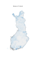
1. The first plot of all the rivers without modifications.
-
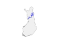
2. The main branch and tributaries.


OSM Geofabrik provides huge amount of GIS data. I need to extract one main branch of that all.
The problems are
- There are many rivers haring the same name
- The shp data breaks
- There are cycles (loops) and tributaries (branches)
1. Plot and check
The analysis of different coordinate systems is shown elsewhere.
Plot all Waterways
import geopandas as gpd
import matplotlib.pyplot as plt

finland = gpd.read_file("fi.shp")
rivers = gpd.read_file("gis_osm_waterways_free_1.shp")

#Check coordinate system
print(finland.crs)
print(rivers.crs) #Says None.
rivers = rivers.set_crs(epsg=4326)
rivers = rivers.to_crs(finland.crs)

#Other coordinate system. Looks even better, more familiar
finland = finland.to_crs(epsg=3067)
rivers = rivers.to_crs(epsg=3067)

#rivers = gpd.clip(rivers, finland) # Clip rivers to Finland

# Plotting
fig, ax = plt.subplots(figsize=(6, 10))
finland.plot( ax=ax, color="#f0f0f0", edgecolor="#444444", linewidth=0.8 )
rivers.plot( ax=ax, color="#4aa3df", linewidth=0.3, alpha=0.7 )

ax.set_axis_off() # Remove axes
plt.title("Rivers of Finland", fontsize=14)
plt.show()
The shp datafile
General format
- .shp = shapes
- .dbf = table (like a spreadsheet with headers)
- .prj = map projection
print(rivers.head())
    osm_id  ...                                           geometry
0  4251428  ...  LINESTRING (384623.065 6671261.378, 384613.062...
1  4336744  ...  LINESTRING (424219.382 6758572.023, 424231.281...
2  4418854  ...  LINESTRING (271969.063 6961997.189, 272511.243...
3  4418989  ...  LINESTRING (263355.182 6994559.516, 263029.852...
4  4494437  ...  LINESTRING (235473.685 6716109.64, 235468.154 ...
print(rivers.columns)
Index(['osm_id', 'code', 'fclass', 'width', 'name', 'geometry'], dtype='object')
print( rivers.info() )
<class 'geopandas.geodataframe.GeoDataFrame'>
RangeIndex: 127503 entries, 0 to 127502
Data columns (total 6 columns):
 #   Column    Non-Null Count   Dtype
---  ------    --------------   -----
 0   osm_id    127503 non-null  object
 1   code      127503 non-null  int32
 2   fclass    127503 non-null  object
 3   width     127503 non-null  int32
 4   name      26074 non-null   object
 5   geometry  127503 non-null  geometry
dtypes: geometry(1), int32(2), object(3)
memory usage: 4.9+ MB
None
print( river( ['fclass'].value_counts() )
fclass
stream    104937
river      12776
drain       9186
canal        604
Name: count, dtype: int64
print(rivers.geometry)
0         LINESTRING (384623.065 6671261.378, 384613.062...
1         LINESTRING (424219.382 6758572.023, 424231.281...
2         LINESTRING (271969.063 6961997.189, 272511.243...
3         LINESTRING (263355.182 6994559.516, 263029.852...
4         LINESTRING (235473.685 6716109.64, 235468.154 ...
                                ...
127498    LINESTRING (193860.594 6771306.041, 193862.48 ...
127499    LINESTRING (193500.06 6770531.712, 193481.661 ...
127500    LINESTRING (267357.405 6823421.996, 267348.152...
127501    LINESTRING (266604.152 6824271.814, 266614.528...
127502    LINESTRING (543881.124 6893248.187, 543974.428...
Name: geometry, Length: 127503, dtype: geometry
print(rivers.describe(include='all'))
        osm_id  ...                                           geometry
count    127503  ...                                             127503
unique   127503  ...                                             127502
top     4251428  ...  LINESTRING (388682.74185180914 6718165.8999426...
freq          1  ...                                                  2
mean        NaN  ...                                                NaN
std         NaN  ...                                                NaN
min         NaN  ...                                                NaN
25%         NaN  ...                                                NaN
50%         NaN  ...                                                NaN
75%         NaN  ...                                                NaN
max         NaN  ...                                                NaN

[11 rows x 6 columns]
gdf['name'].dropna().head(20)
0     Ruoholahdenkanava
1           Porvoonjoki
2            Kyrönjoki
3            Kyrönjoki
4           Raisionjoki
5           Riipinluoma
6             Tjäck Ã¥
7            Kyrönjoki
8            Kyrönjoki
9             Kyro Älv
10            Jalasjoki
11          Kupparinoja
12           Harjunjoki
13         Jyräänjoki
15           Hirvenjoki
16             Takajoki
18             Juotjoki
21     Luhtaanmäenjoki
22         Kostianvirta
23        Ahlaistenjoki
Name: name, dtype: object
2. Plot Kemijoki and tributaries
-

The effect of buffer
-

Larger buffer
-

Clipped with 10 km buffer
-

Clipped with 20 km buffer
-
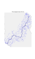
Clipped with 40 km buffer
-
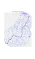
Clipped with 80 km buffer
-

The unary union of the main geometry
-

Connected, intersections
-
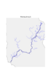
Touching 1. Buffer 80 km.
-

Touching 2. Buffer 80 km.
-

Touching 3. Buffer 80 km.
-
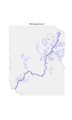
Touching 4. Buffer 80 km.
-

Touching 5. Buffer 80 km.
-

Touching 10. Buffer 80 km.
-

Touching 10. Buffer 80 km.


The beginning (loading the river data files and converting) is the same as before.
kemijoki = rivers[rivers["name"] == "Kemijoki"]
buffer = kemijoki.buffer(50000)  # 20 km buffer around the Kemijoko
buffer_gdf = gpd.GeoDataFrame(geometry=buffer, crs=rivers.crs)

kemijoki_rivers = gpd.clip(rivers, buffer_gdf)

#Find the connected parts
main_geom = unary_union(kemijoki.geometry)
connected = kemijoki_rivers[kemijoki_rivers.geometry.intersects(main_geom)]

current = main_geom
for i in range(5):  # increase if needed
    touching = kemijoki_rivers[kemijoki_rivers.geometry.intersects(current)]
    current = unary_union(touching.geometry)

final_rivers = kemijoki_rivers[kemijoki_rivers.geometry.intersects(current)]

# Plot it
fig, ax = plt.subplots(figsize=(6, 10))

finland.plot(ax=ax, color="#f0f0f0", edgecolor="gray")
final_rivers.plot(ax=ax, color="blue", linewidth=0.4)
kemijoki.plot(ax=ax, color="darkblue", linewidth=1.5)
ax.set_axis_off()

plt.show()
This is easy to edit to show all rivers. However, there are many rivers sharing the same name.
3. Fix the gaps (Make a graph)
Kemijoki_mainbranch.parquet. 4e_combinedByHand.py
4. Plot and check


