Yolo Pose Estimation and Skeleton: Difference between revisions
(→Images) |
|||
| (19 intermediate revisions by the same user not shown) | |||
| Line 29: | Line 29: | ||
import matplotlib.pyplot as plt | import matplotlib.pyplot as plt | ||
import cv2 | import cv2 | ||
from PIL import Image | #from PIL import Image | ||
model = YOLO("yolo11n-pose.pt") # n, s, m, l, x versions available | model = YOLO("yolo11n-pose.pt") # n, s, m, l, x versions available | ||
| Line 39: | Line 39: | ||
plt.axis('off') | plt.axis('off') | ||
plt.imshow(cv2.cvtColor(results[0].plot(), cv2.COLOR_BGR2RGB)) | plt.imshow(cv2.cvtColor(results[0].plot(), cv2.COLOR_BGR2RGB)) | ||
</syntaxhighlight> | |||
The <code>results</code> list includes <code>results[0].keypoints.xy</code>, <code>results[0].keypoints.xyn</code> and <code>results[0].keypoints.conf</code> data. Printing that gives some general information about what is found and how fast, and a <code>tensor</code> vector which includes the position data. | |||
<pre> | |||
image 1/1 /home/mol/Documents/python/skeletor/people2.jpg: 512x640 5 persons, 26.0ms | |||
Speed: 1.4ms preprocess, 26.0ms inference, 38.0ms postprocess per image at shape (1, 3, 512, 640) | |||
tensor([[[1608.5103, 516.1241], | |||
[1600.1213, 497.7412], | |||
[1613.1257, 497.1426], | |||
[1568.5618, 506.6950], | |||
[1648.6650, 505.3312], | |||
[1556.0571, 614.9849], | |||
[1692.7899, 615.2242], | |||
[1540.9780, 763.7505], | |||
[1755.1765, 773.1780], | |||
[1548.3131, 886.3889], | |||
[1795.6322, 892.2405], | |||
[1588.8513, 896.8289], | |||
[1680.1824, 896.3278], | |||
[1574.6792, 1117.8225], | |||
[1675.2017, 1118.2271], | |||
[1589.6167, 1317.0865], | |||
[1671.6086, 1320.7114]], | |||
[[1097.3536, 432.4247], | |||
[1086.8494, 405.5817], | |||
[1092.0603, 402.9798], | |||
[ 987.7101, 409.1143], | |||
[1076.7693, 412.7003], | |||
[ 924.9458, 531.9528], | |||
[1117.5946, 533.4085], | |||
[ 875.2901, 720.3015], | |||
[1186.5740, 715.3069], | |||
[ 862.7459, 861.0502], | |||
[1189.9052, 849.3643], | |||
[ 957.1283, 837.9849], | |||
[1090.0930, 841.1834], | |||
[ 920.7561, 1110.6389], | |||
[1099.1434, 1116.8433], | |||
[ 925.5239, 1367.9281], | |||
[1102.7339, 1381.9753]], | |||
</pre> | |||
To print the coordinates of keypoints, use | |||
<syntaxhighlight lang="python"> | |||
for r in results[0].keypoints.xy: | |||
print(r) | |||
</syntaxhighlight> | |||
Use cv2 to plot the image. This cv2 plotting will be used in the next part. | |||
<syntaxhighlight lang="python"> | |||
image = cv2.imread(filename) | |||
cv2.namedWindow("image", cv2.WINDOW_KEEPRATIO) | |||
cv2.imshow("image", image) | |||
cv2.resizeWindow("image", 600, 600) | |||
cv2.waitKey(0) | |||
cv2.destroyAllWindows() | |||
</syntaxhighlight> | |||
=== CUDA:0 problem === | |||
A CUDA:0 tensor is a tensor that is stored on a GPU, and thus isn't accessible to the CPU. To have it in Numpy, use: | |||
# Copy the data from the GPU to the CPU: `torch.cuda.to_cpu()`. | |||
# Reorder the data (from a column-major format to a row-major): `numpy.transpose()`. Not needed in this simple 1d example. | |||
# Convert the data to NumPy: `numpy.asarray()`, and convert to integer. | |||
<syntaxhighlight lang="python"> | |||
xy_hip =results[0].keypoints.xy[0][12] | |||
cpu_xyhip = np.asarray( xy_hip.cpu() ).astype(np.int64) #Copy and convert; | |||
</syntaxhighlight> | </syntaxhighlight> | ||
=== Pose to skeleton === | === Pose to skeleton === | ||
The keypoint coordinates need to be converted to bones; as an example, femur is located between | |||
* 12 (left hip) and 14 (left knee) or | |||
* 13 (right hip) and 15 (right knee) | |||
First, plot a line between the joints: | |||
<syntaxhighlight lang="python"> | |||
xy_knee = results[0].keypoints.xy[0][14] | |||
xyknee = np.asarray( xy_knee.cpu() ).astype(np.int64) | |||
xy_hip =results[0].keypoints.xy[0][12] | |||
xyhip = np.asarray( xy_hip.cpu() ).astype(np.int64) #Copy and convert; | |||
cv2.line( image, xyhip , xyknee, (0,250,0), 9) | |||
</syntaxhighlight> | |||
Then, get the angle and insert the image of the bone instead. | |||
=== Combine/ blend images === | |||
Pillow, cv2, Scikit-image. | |||
* https://stackoverflow.com/questions/55795755/how-to-add-an-image-over-another-image-using-x-y-coordinates | |||
PIL | |||
* <code>Image.Image.paste(im1, im2, (50, 125))</code> | |||
* <code>im1 = im1.rotate(90, PIL.Image.NEAREST, expand = 1)</code> | |||
PIL and cv2 | |||
<syntaxhighlight lang="python"> | |||
pil_im = Image.open("image.jpg") | |||
cv_im = cv2.cvtColor(np.array(pil_im), cv2.COLOR_RGB2BGR) | |||
# Apply OpenCV operations | |||
edges = cv2.Canny(cv_im, 100, 200) | |||
# Convert back to PIL and display | |||
pil_edges = Image.fromarray(edges) | |||
pil_edges.show() | |||
</syntaxhighlight> | |||
=== === | === === | ||
== Images == | == Images == | ||
=== 1 === | |||
Scale the image height to 400 px and width such that the center of bone is in the middle of the image. | |||
=== 2 === | |||
=== 3 === | |||
== Video == | == Video == | ||
| Line 52: | Line 174: | ||
* https://medium.com/@staytechrich/human-pose-estimation-with-yolov11-96932a5d7159 | * https://medium.com/@staytechrich/human-pose-estimation-with-yolov11-96932a5d7159 | ||
* https://www.labellerr.com/blog/how-to-perform-yolos-various-task/ | |||
* https://www.bomberbot.com/python/mastering-pythons-pil-image-show-method-a-deep-dive-for-developers/ | |||
Latest revision as of 21:00, 7 October 2025
Introduction
Make a pose estimator and use it to make a moving skeleton.
Use Yolo from Ultralytics.
- Python 3.7+
- Yolo v11
- A CUDA-enabled GPU (optional but recommended for faster inference).
pip install ultralytics opencv-python numpy
Yolo
There are 17 keypoints. YOLOv11’s pose model outputs:
- (x, y) coordinates for each keypoint and
- confidence scores indicating the model’s certainty in each keypoint’s position.
Image detection
-
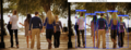
AN image before and after the code.
from ultralytics import YOLO
import matplotlib.pyplot as plt
import cv2
#from PIL import Image

model = YOLO("yolo11n-pose.pt")  # n, s, m, l, x versions available

results = model.predict(source="sample_image.jpg")

plt.figure(figsize=(10, 10))
plt.title('YOLOv11 Pose Results')
plt.axis('off')
plt.imshow(cv2.cvtColor(results[0].plot(), cv2.COLOR_BGR2RGB))
The results list includes results[0].keypoints.xy, results[0].keypoints.xyn and results[0].keypoints.conf data. Printing that gives some general information about what is found and how fast, and a tensor vector which includes the position data.
image 1/1 /home/mol/Documents/python/skeletor/people2.jpg: 512x640 5 persons, 26.0ms
Speed: 1.4ms preprocess, 26.0ms inference, 38.0ms postprocess per image at shape (1, 3, 512, 640)
tensor([[[1608.5103,  516.1241],
         [1600.1213,  497.7412],
         [1613.1257,  497.1426],
         [1568.5618,  506.6950],
         [1648.6650,  505.3312],
         [1556.0571,  614.9849],
         [1692.7899,  615.2242],
         [1540.9780,  763.7505],
         [1755.1765,  773.1780],
         [1548.3131,  886.3889],
         [1795.6322,  892.2405],
         [1588.8513,  896.8289],
         [1680.1824,  896.3278],
         [1574.6792, 1117.8225],
         [1675.2017, 1118.2271],
         [1589.6167, 1317.0865],
         [1671.6086, 1320.7114]],

        [[1097.3536,  432.4247],
         [1086.8494,  405.5817],
         [1092.0603,  402.9798],
         [ 987.7101,  409.1143],
         [1076.7693,  412.7003],
         [ 924.9458,  531.9528],
         [1117.5946,  533.4085],
         [ 875.2901,  720.3015],
         [1186.5740,  715.3069],
         [ 862.7459,  861.0502],
         [1189.9052,  849.3643],
         [ 957.1283,  837.9849],
         [1090.0930,  841.1834],
         [ 920.7561, 1110.6389],
         [1099.1434, 1116.8433],
         [ 925.5239, 1367.9281],
         [1102.7339, 1381.9753]],
To print the coordinates of keypoints, use
for r in results[0].keypoints.xy:
    print(r)
Use cv2 to plot the image. This cv2 plotting will be used in the next part.
image = cv2.imread(filename)

cv2.namedWindow("image", cv2.WINDOW_KEEPRATIO)
cv2.imshow("image", image)
cv2.resizeWindow("image", 600, 600)
cv2.waitKey(0)
cv2.destroyAllWindows()
CUDA:0 problem
A CUDA:0 tensor is a tensor that is stored on a GPU, and thus isn't accessible to the CPU. To have it in Numpy, use:
- Copy the data from the GPU to the CPU: `torch.cuda.to_cpu()`.
- Reorder the data (from a column-major format to a row-major): `numpy.transpose()`. Not needed in this simple 1d example.
- Convert the data to NumPy: `numpy.asarray()`, and convert to integer.
xy_hip =results[0].keypoints.xy[0][12]
cpu_xyhip = np.asarray( xy_hip.cpu() ).astype(np.int64) #Copy and convert;
Pose to skeleton
The keypoint coordinates need to be converted to bones; as an example, femur is located between
- 12 (left hip) and 14 (left knee) or
- 13 (right hip) and 15 (right knee)
First, plot a line between the joints:
xy_knee = results[0].keypoints.xy[0][14]
xyknee = np.asarray( xy_knee.cpu() ).astype(np.int64)

xy_hip =results[0].keypoints.xy[0][12]
xyhip = np.asarray( xy_hip.cpu() ).astype(np.int64) #Copy and convert;

cv2.line( image, xyhip , xyknee, (0,250,0), 9)
Then, get the angle and insert the image of the bone instead.
Combine/ blend images
Pillow, cv2, Scikit-image.
PIL
Image.Image.paste(im1, im2, (50, 125))im1 = im1.rotate(90, PIL.Image.NEAREST, expand = 1)
PIL and cv2
pil_im = Image.open("image.jpg")
cv_im = cv2.cvtColor(np.array(pil_im), cv2.COLOR_RGB2BGR)

# Apply OpenCV operations
edges = cv2.Canny(cv_im, 100, 200)

# Convert back to PIL and display
pil_edges = Image.fromarray(edges)
pil_edges.show()
Images
1
Scale the image height to 400 px and width such that the center of bone is in the middle of the image.