Python and phyphox: Difference between revisions
| (54 intermediate revisions by the same user not shown) | |||
| Line 3: | Line 3: | ||
=== VIM | === Phyphox XML and VIM === | ||
Activate the matchit.vim macro <code>:runtime macros/matchit.vim</code> and set the filetype <code>:set filetype=html</code> (or xml), and now % swaps between the tags. | Activate the matchit.vim macro <code>:runtime macros/matchit.vim</code> and set the filetype <code>:set filetype=html</code> (or xml), and now % swaps between the tags. | ||
The data is located in <code><data-containers></code> blocks and <code><container></code> tag contains the data of each measurements. | The data is located in <code><data-containers></code> blocks and <code><container></code> tag contains the data of each measurements, but is in <code>init</code> tag, as shown below: <code><container size="0" init="1.009771156E1,1.012672424E1,1.004746246E1,1.009292603E1,1.024636555E1,1.024875832E1,1.015065289E1,1.007617569E1,1.012193871E1,1.011954594E1,9.999606133E0,9.978070259E0,1.0059426</code>. Thus, we need to read the init part only. | ||
=== Load the acceleration data === | |||
The simplest | |||
<syntaxhighlight lang="python"> | |||
import pandas as pd | |||
df = pd.read_xml( filename ) | |||
</syntaxhighlight> | |||
does not work if the XML file is too large. Use lxml from etree instead: | |||
<syntaxhighlight lang="python"> | |||
from lxml import etree | |||
def parse_lxml_large_xml(source, a): | |||
for event, elem in etree.iterparse(source, events=('end',)): | |||
if elem.tag == "container" and elem.text == a: | |||
#Split the string and convert to float | |||
A = elem.text | |||
B = elem.attrib | |||
BB = B.get('init').split(",") | |||
data = np.empty( (len( BB ), 1 ) ) | |||
for i, d in enumerate( BB ): | |||
data[i,0] = float(d) | |||
elem.clear() # Free memory | |||
return data | |||
</syntaxhighlight> | |||
and use it as | |||
<syntaxhighlight lang="python"> | |||
accX = parse_lxml_large_xml( "nousu_waw_tll_edited.phyphox", "accX" ) | |||
accY = parse_lxml_large_xml( "nousu_waw_tll_edited.phyphox", "accY" ) | |||
accZ = parse_lxml_large_xml( "nousu_waw_tll_edited.phyphox", "accZ" ) | |||
acc = parse_lxml_large_xml( "nousu_waw_tll_edited.phyphox", "acc" ) | |||
time = parse_lxml_large_xml( "nousu_waw_tll_edited.phyphox", "acc_time" ) | |||
A = np.column_stack( [time, accX, accY, accZ, acc] ) | |||
df = pd.DataFrame( A, columns=['time', 'ax', 'ay', 'az', 'a'] ) | |||
df.set_index('time', inplace=True) | |||
</syntaxhighlight> | |||
The last line changes the time column to be the index column, and the <code>inplace</code> keyword replaces that data directly into <code>df</code> variable. | |||
We can load any other data similarly, too. Just change the the names in function calls. | |||
== Flights == | == Flights == | ||
=== 1. Departure WAW-TLL === | === 1. Departure WAW-TLL: Plot the data === | ||
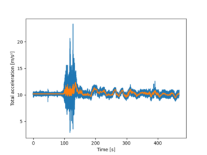
[[File:Phyphox Flight waw-tll draw1.png|thumb|The raw total acceleration data with rolling mean]] | |||
<syntaxhighlight lang="python"> | |||
ax = df.a.plot() | |||
ax = df.a.rolling(window=100).mean().plot(x='time') | |||
ax.set_xlabel('Time [s]') | |||
ax.set_ylabel("Total acceleration [m/s²]") | |||
plt.show() | |||
</syntaxhighlight> | |||
The <code>rolling(window=100).mean()</code> calculates the rolling mean with a window of width 100 to be plotted. The <code>x='time'</code> in parenthesis is not obligatory, as we already stated that the index is time. The two lines are to state the x and y labels better. The final line is to show the image. | |||
The command | |||
<syntaxhighlight lang="python"> | |||
ax.legend(['All data', 'Rolling mean (100)'] ) | |||
plt.show() | |||
</syntaxhighlight> | |||
will give the legend box. Note that the <code>plt.show()</code> need to be added here. | |||
''It is clearly shown that the something happens about at t=96 s; the acceleration changes from a bit over 10 to something else. However, even the smoothed data is rather difficult to visualize what happens.'' | |||
=== 1. Departure WAW-TLL: Check the Rolling mean === | |||
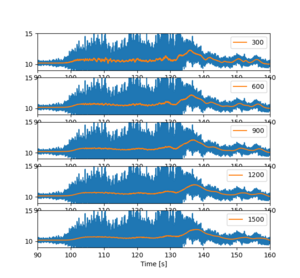
[[File:Phyphox Flight waw-tll draw2 subfigures.png|thumb|Different rolling window sizes]] | |||
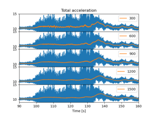
[[File:Phyphox Flight waw-tll draw2b subfiguresadjusted.png|thumb|Adjust the separation between subfigures]] | |||
We need to check if the size of the window in the rolling gives different and perhaps easily interpreted figures. | |||
<syntaxhighlight lang="python"> | |||
fig = plt.figure() | |||
for i in range(1,6): | |||
ax = fig.add_subplot(5,1,i) | |||
df.a.plot( label='_nolegend_' ) | |||
df.a.rolling(window=i*300).mean().plot(x='time') | |||
ax.set_xlim([90,160]) | |||
ax.set_ylim([9,15]) | |||
ax.set_xlabel('Time [s]') | |||
ax.legend( [str(i*300) ] ) | |||
plt.show() | |||
</syntaxhighlight > | |||
To loop many values, use <code>for</code> syntax. Set the limits to <code>x</code> and <code>y</code> axis to help visualize the data better. Also depict in the legend what is the window size. The legend of the original (blue) line is not shown, because its label is stated <code>_nolegend</code>. | |||
The xlabels are are partly hidden below the images, and there is some empty space between the subfigure panels. We could remove those, but the zooming becomes difficult as the different subfigures zoom at different rates. but for printing purposes that would be good option. | |||
Thus add the following commands to be end of the for loop: | |||
<syntaxhighlight lang="python"> | |||
if i<5: | |||
ax.set_xticks([]) | |||
if i==1: | |||
ax.set_title('Total acceleration') | |||
plt.subplots_adjust(hspace=0.) | |||
</syntaxhighlight > | |||
Don't forget to the <code>plt.show()</code> command. | |||
''We note that though the rolling mean is about similar in all the cases, the larger is better. Next we will study the acceleration in different axes.'' | |||
=== 1. Departure WAW-TLL: Analyze the acceleration along axes === | |||
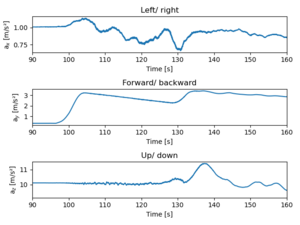
[[File:Phyphox Flight waw-tll draw3acceleration.png|thumb|Acceleration with smoothed data is looking good.]] | |||
[[File:Phyphox Flight waw-tll draw4velocity.png|thumb|Integrated velocity]] | |||
The acceleration axes are following: | |||
* a<sub>x</sub> left/ right | |||
* a<sub>y</sub> forward/ backward | |||
* a<sub>z</sub> up/ down | |||
Create the image, then add subplots and plot. | |||
<syntaxhighlight lang="python"> | |||
fig = plt.figure() | |||
</syntaxhighlight> | |||
Only the last is shown here: | |||
<syntaxhighlight lang="python"> | |||
ax3 = fig.add_subplot(3,1,3) | |||
df.az.rolling(window=1200).mean().plot() | |||
ax3.set_xlim([90,160]) | |||
ax3.set_xlabel('Time [s]') | |||
ax3.set_ylabel('a$_z$ [m/s²]') | |||
ax3.set_title('Up/ down') | |||
plt.tight_layout() | |||
plt.show() | |||
</syntaxhighlight> | |||
''The plane starts accelerating at t=96.5 seconds, and accelerates smoothly until t=128 when something happened. Perhaps the front wheels lifted off the ground. At t=132 secs the z acceleration shows a bump starting, and that must depict that the plane was lifted. At the same time some small steering manouvers was done, and the forward acceleration was increased. Either there was more poer or the frictional drag force due to the wheels is smaller.'' | |||
The acceleration is too big. This might be due to the non-orthogonal orientation of the mobile phone while measuring. Thus, we'll need to check the phone angle. However, the line is so smooth that let's try to integrate the acceleration to get the speed. There multiple different integration methods, and we will use trapezoid method implemented in the Python. | |||
<syntaxhighlight lang="python"> | |||
from scipy import integrate | |||
fig = plt.figure() | |||
#Mask the data and plot the original | |||
mask = (df.index>=90) & (df.index<=160) | |||
ax1 = fig.add_subplot(2,1,1) | |||
dfmasked=pd.DataFrame() | |||
dfmasked["ay"] = df[mask].ay.rolling(window=1200).mean().dropna() | |||
df[mask].ay.rolling(window=1200).mean().plot() | |||
ax1.set_ylim([0,3.5]) | |||
ax1.set_title('Acceleration') | |||
ax1.set_ylabel("Acceleration [m/s²]") | |||
#Calculate the integral; drop the nans first | |||
dfmasked.dropna(inplace=True) | |||
dfmasked["vy"] = integrate.cumulative_trapezoid(dfmasked.ay, dfmasked.index, initial=0) | |||
ax2 = fig.add_subplot(2,1,2) | |||
dfmasked.vy.plot() | |||
ax2.set_ylim([0,190]) | |||
ax2.set_title('Velocity') | |||
ax2.set_ylabel("Speed [m/s]") | |||
plt.tight_layout() | |||
plt.show() | |||
</syntaxhighlight> | |||
The data is first masked into correct location, as the numerical integration is not very stable. Then, the data is smoothed via the same method as earlier, and plotter. | |||
Furthermore, we plotted the turning points, or local extrema. Those datapoints were found by looking the data as the algorithms for the numerical extrema work not that good if the the data is noisy. | |||
<syntaxhighlight lang="python"> | |||
lines = [97, 104, 129, 134, 137, 141, 144, 150, 152] | |||
for l in lines: | |||
plt.plot( [l, l], [-1, 4], 'k', alpha=0.1 ) | |||
</syntaxhighlight> | |||
The third part consists of integrating the y-direction of the acceleration. Before, we need to drop the NaNs that occur because of the rolling mean. Again, the image is plotted and the lines are shown. | |||
''We note that the the speed increases till t=129 when then lift off happens at speed 82 m/s or 300 km/h. The typical lift off velocities are 241 km/h (Boeing 737) or 274 km/h (Airbus A320), thus the result is somehow reasonable.'' | |||
=== Departure WAW-TLL: Linearize the data === | |||
The acceleration data is almost linear, so lets do a small regression analysis to get a bit simpler model. The complication is that the regression model should be piecewise continuous. There are automatic methods (eg linear tree, see https://gist.github.com/ruoyu0088/70effade57483355bbd18b31dc370f2a) but we will use semi-manual system using the <code>plwf</code> library https://jekel.me/piecewise_linear_fit_py/examples.html. One option would be to assign a piecewise function in numpy, and then fit the data into the function, but there is an easier solution, by using pwlf library. | |||
[[File:Phyphox Flight waw-tll draw5b piecewiseLinearFit.png|thumb|Piecewise linear fit]] | |||
'''Piecewise linear fit''' (<code>plwf</code> library) is easy to use, but somehow it doesn't follow all the points, as is shown on the Figure. | |||
<syntaxhighlight lang="python"> | |||
import pwlf | |||
df_rolled = df.ax.rolling(window=1200).mean().dropna() | |||
xs = np.array([0, 99, 104, 109, 112.5, 116, 117, 118.5, 120, 127, 130, 135, 145, 160]) | |||
my_pwlf = pwlf.PiecewiseLinFit(df_rolled.index.values, df_rolled.values ) | |||
my_pwlf.fit_with_breaks(xs) | |||
xHat = np.linspace(0, 160, num=10000) | |||
yHat = my_pwlf.predict(xHat) | |||
plt.plot(xHat, yHat, '-') | |||
</syntaxhighlight> | |||
[[File:Phyphox Flight waw-tll draw5d piecewiseLinearFit simple.png|thumb|Hand-made linear fit with no optimization. Works rather well.]] | |||
<syntaxhighlight lang="python"> | |||
df_rolled = df.ax.rolling(window=1200).mean().dropna() | |||
xs = np.array([0, 99, 104, 109, 112.5, 116, 117, 118.5, 120, 127, 130, 135, 145, 160]) | |||
ys = np.empty( np.shape(xs) ) | |||
for i, time in enumerate(xs): | |||
X = df_rolled.loc[ int(time):] | |||
ys[i] = X.iloc[0] | |||
for i in range(1, np.shape(xs)[0]): | |||
plt.plot( [xs[i-1], xs[i]], [ys[i-1], ys[i]], 'r' ) | |||
</syntaxhighlight > | |||
[[File:Phyphox Flight waw-tll draw5c piecewiseLinearFit fulloptimization.png|thumb|Automatically find the points.]] | |||
'''Piecewise linear fit''' with optimization, does not work very well. This should be with 8 segments but only five is seen. | |||
<code> | |||
res = my_pwlf.fit(8) | |||
</code> | |||
'''Piecewise linear fit''' with forcing through data points does not converge. It says only <code> LinAlgWarning: Ill-conditioned matrix (rcond=7.2053e-35): result may not be accurate</code> but tries to optimize. | |||
<syntaxhighlight lang="python"> | |||
ys = np.empty( np.shape(xs) ) | |||
for i, time in enumerate(xs): | |||
X = df_rolled.loc[ int(time): ] | |||
ys[i] = X.iloc[0].ax | |||
res = my_pwlf.fit( np.shape( xs )[0], xs, ys ) | |||
</syntaxhighlight> | |||
[[File:Phyphox Flight waw-tll draw5a piecewise.png|thumb|Simple piecewise nut not continous function]] | |||
'''Piecewise''' function is not continous. This is a failed attemp. The following code assumes that the piecewise points are known. The <code>linear_model</code> needs the data in a strange format, and thus the <code>reshape</code> command is used. | |||
<syntaxhighlight lang="python"> | |||
from sklearn import datasets, linear_model | |||
xs = np.array([0, 99, 104, 109, 112.5, 116, 117, 118.5, 120, 127, 130, 135, 145, 160]) | |||
for i in range(1, np.shape(xs)[0]): | |||
X = df.loc[ xs[i-1]:xs[i] ] | |||
regr = linear_model.LinearRegression() | |||
regr.fit( X.index.values.reshape(-1,1), X.ax.values.reshape(-1,1) ) | |||
ax1.plot( X.index.values.reshape(-1,1), regr.predict( X.index.values.reshape(-1,1) ), color='red' ) | |||
</syntaxhighlight> | |||
=== Departure WAW-TLL: Check the angle of the phone and plane === | |||
The phone (measuring device) was located on the bench, and thus it is not oriented orthogonal according to the gravitation force. | |||
=== === | === === | ||
Latest revision as of 17:52, 16 June 2025
Introduction
Phyphox XML and VIM
Activate the matchit.vim macro :runtime macros/matchit.vim and set the filetype :set filetype=html (or xml), and now % swaps between the tags.
The data is located in <data-containers> blocks and <container> tag contains the data of each measurements, but is in init tag, as shown below: <container size="0" init="1.009771156E1,1.012672424E1,1.004746246E1,1.009292603E1,1.024636555E1,1.024875832E1,1.015065289E1,1.007617569E1,1.012193871E1,1.011954594E1,9.999606133E0,9.978070259E0,1.0059426. Thus, we need to read the init part only.
Load the acceleration data
The simplest
import pandas as pd
df = pd.read_xml( filename )
does not work if the XML file is too large. Use lxml from etree instead:
from lxml import etree

def parse_lxml_large_xml(source, a):
    for event, elem in etree.iterparse(source, events=('end',)):
        if elem.tag == "container" and elem.text == a:
            #Split the string and convert to float
            A = elem.text
            B = elem.attrib
            BB = B.get('init').split(",")
            data = np.empty( (len( BB  ), 1 ) )
            for i, d in enumerate( BB ):
                data[i,0] = float(d)
            elem.clear()  # Free memory
    return data
and use it as
accX = parse_lxml_large_xml( "nousu_waw_tll_edited.phyphox", "accX" )
accY = parse_lxml_large_xml( "nousu_waw_tll_edited.phyphox", "accY" )
accZ = parse_lxml_large_xml( "nousu_waw_tll_edited.phyphox", "accZ" )
acc = parse_lxml_large_xml( "nousu_waw_tll_edited.phyphox", "acc" )
time = parse_lxml_large_xml( "nousu_waw_tll_edited.phyphox", "acc_time" )

A = np.column_stack( [time, accX, accY, accZ, acc]  )
df = pd.DataFrame( A, columns=['time', 'ax', 'ay', 'az', 'a'] )
df.set_index('time', inplace=True)
The last line changes the time column to be the index column, and the inplace keyword replaces that data directly into df variable.
We can load any other data similarly, too. Just change the the names in function calls.
Flights
1. Departure WAW-TLL: Plot the data
ax = df.a.plot()
ax = df.a.rolling(window=100).mean().plot(x='time')
ax.set_xlabel('Time [s]')
ax.set_ylabel("Total acceleration [m/s²]")
plt.show()
The rolling(window=100).mean() calculates the rolling mean with a window of width 100 to be plotted. The x='time' in parenthesis is not obligatory, as we already stated that the index is time. The two lines are to state the x and y labels better. The final line is to show the image.
The command
ax.legend(['All data', 'Rolling mean (100)'] )
plt.show()
will give the legend box. Note that the plt.show() need to be added here.
It is clearly shown that the something happens about at t=96 s; the acceleration changes from a bit over 10 to something else. However, even the smoothed data is rather difficult to visualize what happens.
1. Departure WAW-TLL: Check the Rolling mean
We need to check if the size of the window in the rolling gives different and perhaps easily interpreted figures.
fig = plt.figure()
for i in range(1,6):
    ax = fig.add_subplot(5,1,i)
    df.a.plot( label='_nolegend_' )
    df.a.rolling(window=i*300).mean().plot(x='time')
    ax.set_xlim([90,160])
    ax.set_ylim([9,15])
    ax.set_xlabel('Time [s]')
    ax.legend( [str(i*300) ] )
plt.show()
To loop many values, use for syntax. Set the limits to x and y axis to help visualize the data better. Also depict in the legend what is the window size. The legend of the original (blue) line is not shown, because its label is stated _nolegend.
The xlabels are are partly hidden below the images, and there is some empty space between the subfigure panels. We could remove those, but the zooming becomes difficult as the different subfigures zoom at different rates. but for printing purposes that would be good option.
Thus add the following commands to be end of the for loop:
    if i<5:
        ax.set_xticks([])
    if i==1:
        ax.set_title('Total acceleration')
plt.subplots_adjust(hspace=0.)
Don't forget to the plt.show() command.
We note that though the rolling mean is about similar in all the cases, the larger is better. Next we will study the acceleration in different axes.
1. Departure WAW-TLL: Analyze the acceleration along axes
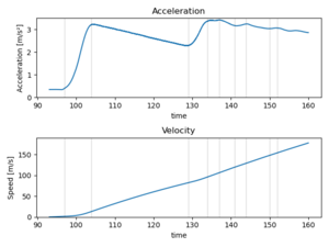
The acceleration axes are following:
- ax left/ right
- ay forward/ backward
- az up/ down
Create the image, then add subplots and plot.
fig = plt.figure()
Only the last is shown here:
ax3 = fig.add_subplot(3,1,3)
df.az.rolling(window=1200).mean().plot()
ax3.set_xlim([90,160])
ax3.set_xlabel('Time [s]')
ax3.set_ylabel('a$_z$ [m/s²]')
ax3.set_title('Up/ down')

plt.tight_layout()

plt.show()
The plane starts accelerating at t=96.5 seconds, and accelerates smoothly until t=128 when something happened. Perhaps the front wheels lifted off the ground. At t=132 secs the z acceleration shows a bump starting, and that must depict that the plane was lifted. At the same time some small steering manouvers was done, and the forward acceleration was increased. Either there was more poer or the frictional drag force due to the wheels is smaller.
The acceleration is too big. This might be due to the non-orthogonal orientation of the mobile phone while measuring. Thus, we'll need to check the phone angle. However, the line is so smooth that let's try to integrate the acceleration to get the speed. There multiple different integration methods, and we will use trapezoid method implemented in the Python.
from scipy import integrate
fig = plt.figure()

#Mask the data and plot the original
mask = (df.index>=90) & (df.index<=160)

ax1 = fig.add_subplot(2,1,1)
dfmasked=pd.DataFrame()
dfmasked["ay"] = df[mask].ay.rolling(window=1200).mean().dropna()
df[mask].ay.rolling(window=1200).mean().plot()

ax1.set_ylim([0,3.5])
ax1.set_title('Acceleration')
ax1.set_ylabel("Acceleration [m/s²]")


#Calculate the integral; drop the nans first
dfmasked.dropna(inplace=True)
dfmasked["vy"] = integrate.cumulative_trapezoid(dfmasked.ay, dfmasked.index, initial=0)

ax2 = fig.add_subplot(2,1,2)
dfmasked.vy.plot()

ax2.set_ylim([0,190])
ax2.set_title('Velocity')
ax2.set_ylabel("Speed [m/s]")

plt.tight_layout()
plt.show()
The data is first masked into correct location, as the numerical integration is not very stable. Then, the data is smoothed via the same method as earlier, and plotter.
Furthermore, we plotted the turning points, or local extrema. Those datapoints were found by looking the data as the algorithms for the numerical extrema work not that good if the the data is noisy.
lines = [97, 104, 129, 134, 137, 141, 144, 150, 152]
for l in lines:
    plt.plot( [l, l], [-1, 4], 'k', alpha=0.1  )
The third part consists of integrating the y-direction of the acceleration. Before, we need to drop the NaNs that occur because of the rolling mean. Again, the image is plotted and the lines are shown.
We note that the the speed increases till t=129 when then lift off happens at speed 82 m/s or 300 km/h. The typical lift off velocities are 241 km/h (Boeing 737) or 274 km/h (Airbus A320), thus the result is somehow reasonable.
Departure WAW-TLL: Linearize the data
The acceleration data is almost linear, so lets do a small regression analysis to get a bit simpler model. The complication is that the regression model should be piecewise continuous. There are automatic methods (eg linear tree, see https://gist.github.com/ruoyu0088/70effade57483355bbd18b31dc370f2a) but we will use semi-manual system using the plwf library https://jekel.me/piecewise_linear_fit_py/examples.html. One option would be to assign a piecewise function in numpy, and then fit the data into the function, but there is an easier solution, by using pwlf library.
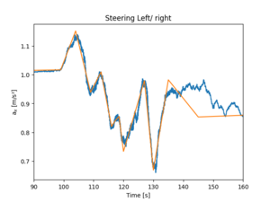
Piecewise linear fit (plwf library) is easy to use, but somehow it doesn't follow all the points, as is shown on the Figure.
import pwlf
df_rolled = df.ax.rolling(window=1200).mean().dropna()

xs = np.array([0, 99, 104, 109, 112.5, 116, 117, 118.5, 120, 127, 130, 135, 145, 160])

my_pwlf = pwlf.PiecewiseLinFit(df_rolled.index.values, df_rolled.values )
my_pwlf.fit_with_breaks(xs)
xHat = np.linspace(0, 160, num=10000)
yHat = my_pwlf.predict(xHat)
plt.plot(xHat, yHat, '-')
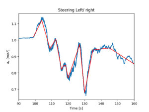
df_rolled = df.ax.rolling(window=1200).mean().dropna()
xs = np.array([0, 99, 104, 109, 112.5, 116, 117, 118.5, 120, 127, 130, 135, 145, 160])
ys = np.empty( np.shape(xs) )
for i, time in enumerate(xs):
    X = df_rolled.loc[ int(time):]
    ys[i] = X.iloc[0]
for i in range(1, np.shape(xs)[0]):
    plt.plot( [xs[i-1], xs[i]], [ys[i-1], ys[i]], 'r'  )
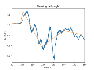
Piecewise linear fit with optimization, does not work very well. This should be with 8 segments but only five is seen.
res = my_pwlf.fit(8)
Piecewise linear fit with forcing through data points does not converge. It says only LinAlgWarning: Ill-conditioned matrix (rcond=7.2053e-35): result may not be accurate but tries to optimize.
ys = np.empty( np.shape(xs) )
for i, time in enumerate(xs):
    X = df_rolled.loc[ int(time): ]
    ys[i] = X.iloc[0].ax
res = my_pwlf.fit( np.shape( xs )[0], xs, ys )
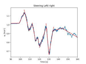
Piecewise function is not continous. This is a failed attemp. The following code assumes that the piecewise points are known. The linear_model needs the data in a strange format, and thus the reshape command is used.
from sklearn import datasets, linear_model
xs = np.array([0, 99, 104, 109, 112.5, 116, 117, 118.5, 120, 127, 130, 135, 145, 160])

for i in range(1, np.shape(xs)[0]):
    X = df.loc[ xs[i-1]:xs[i] ]

    regr = linear_model.LinearRegression()
    regr.fit( X.index.values.reshape(-1,1), X.ax.values.reshape(-1,1) )
    ax1.plot( X.index.values.reshape(-1,1), regr.predict( X.index.values.reshape(-1,1)  ), color='red'  )
Departure WAW-TLL: Check the angle of the phone and plane
The phone (measuring device) was located on the bench, and thus it is not oriented orthogonal according to the gravitation force.